In real-life scenarios, we often face scenarios where we need to plot data with higher-order dimensions. For example, suppose we want to plot any object’s space coordinates over some time interval in the time-varying magnetic or electric field. We will need the three-dimensional plots to describe the object’s coordinates perfectly. The scatter plot is a kind of plot in which we plot the discrete data points in the figure that are not connected. When we plot the scatter plot in three-dimensional space, it is known as three dimensional scatter plot. This article will explain how to plot to scatter plots in three-dimensional space in python matplotlib.

How to Create a Three-Dimensional (3D) Figure in Matplotlib?

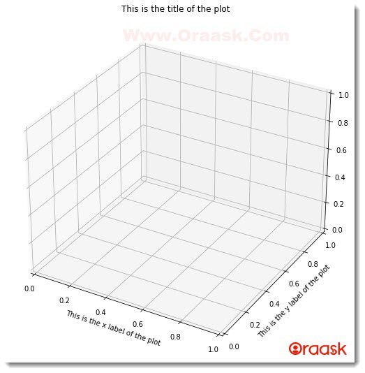
Before we plot the three-dimensional scatter plot in matplotlib, it is important to understand how to plot the three-dimensional figure in matplotlib. For creating the three-dimensional workspace in matplotlib, we first create a 3-D object using the following lines of codes:

ax=plt.axes(projection=”3d”)

Note that the user can change the variable name ax since it is not any keyword or user-defined function. Also, plt is an alias name for matplotlib.pyplot.We can add titles, labels, figure size, etc., to the plots using the functions we used in the case of two-dimensional figures.

Example (1)

#import all the necessary libraries and modules
import numpy as np
import matplotlib.pyplot as plt
#create the main() function
def main():
    #creating the figure class 
    fig=plt.figure(figsize=(9,9))
    #creating the three-dimensional axes
    ax=plt.axes(projection="3d")
    #defining title to the plot
    plt.title("This is the title of the plot")
    #defining the label along the x-axis
    plt.xlabel("This is the x label of the plot")
    #defining the label along the y axis
    plt.ylabel("This is the y label of the plot")
    #displaying the plot
    plt.show()
#calling the main() function
if __name__ == "__main__":
    main ()

Output:

Explanation:

1. First, as customary, we have imported the libraries and packages in the code. We have imported two libraries, namely numpy and the matplotlib.pyplot.We used alias names for our convenience in writing the codes.
2. Next, we created the main() function in the code. Under the function, we first changed the figure size of our plot using the following code:

fig=plt.figure(figsize=(9,9))

Note that the figure attribute takes tuples as the input. The user can change the value (9,9).

3. After that, we have defined the title,labels to the figure using the title() function,xlabel() ,ylabel() function.Finaly we displayed the graph using the plt.show() function.Note that this is optional to add the plt.show() code fot Jupyter Notebook.
4. Finally, we declared the main() function as the main driving code of the program using the following lines of code:

if __name__ == “__main__”:

    main ()

Plotting a Simple Three-Dimensional (3D) Scatter Plot in Matplotlib

Now we are in a position to plot simple three-dimensional scatter plots in matplotlib.

We need to keep in mind the following points to plot the three-dimensional scatter plot:

1. We must define data points for three axes in the code.
2. We have to pass a minimum of three parameters to the 3-D plot.
3. We can use all other functions associated with the two-dimensional scatter plot.
4. Dimensions of all the data points along the three axes should be the same. For example, if the x has 30 data points, then y and z must have 30 data points, too, in the code.
5. The values of the data points should be in the form of a numpy like an object, array, list, etc., data types.

Example (2)

#import all the necessary libraries
import numpy as np
import matplotlib.pyplot as plt

#defining a user-defined function to plot the three-dimensional scatter plot
def three_dimensional_scatter(x,y,z):
    #creating figure object in the plot
    fig = plt.figure(figsize = (9,9))
    #created three-dimensional workspace 
    ax = plt.axes(projection ="3d")
    #plotting the three-dimensional scatter plot using the parameters 
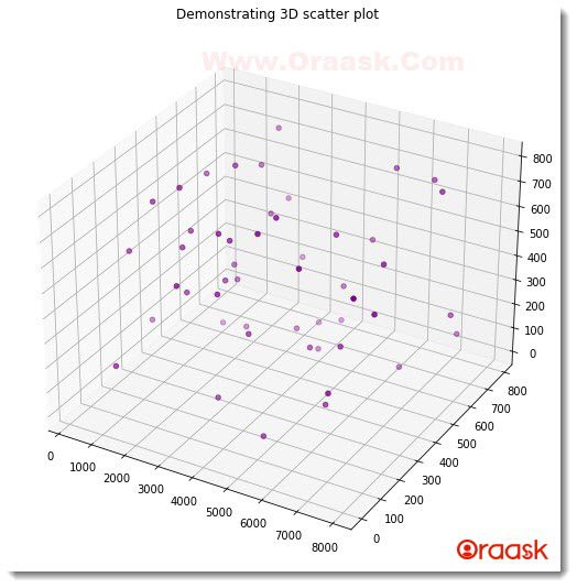
    ax.scatter3D(x, y, z, color = "purple")
    #defining title to the plot
    plt.title("Demonstrating 3D scatter plot")
    #displaying the three-dimensional scatter plot
    plt.show()
    
#creating the main() function
def main():
    #creating data points for the z-axis
    z = np.random.randint(800, size =(50))
    print(f"Z values generated are: {z}")
    #creating data points for the x-axis
    x = np.random.randint(8000, size =(50))
    print(f"x values generated are: {x}")
    #creating data points for the y axis
    y = np.random.randint(800, size =(50))
    print(f"y values generated are: {y}")
    #calling the main() function
    three_dimensional_scatter(x,y,z)

#callng the main() function
if __name__ == "__main__":
    main()

Output:

Z values generated are: [ 27 279 129 797 418 313 428 115 755 730 231 503 281 727 622 703 560 603

 299 273 657 744 792  12 742 686 567  80 113 774 181   4 639 244 399 441

 508 702 778 320 105  26 373 700  68 577   4   2 510 678]

x values generated are: [3967 6880  256 1864 2753 6264 2009 3678 7387 5630 2663  414 7765 1854

 7072 6605 2788 1916 3877 4626 5542 7955 4725 3414 6124 1249 1936 2270

 7431 4585 4847 1143 3277 1455 2098 5126 3531 3281 2321 2353 6108 6428

 2232  963 3371 7771 4027 4907 2585 2171]

y values generated are: [731 124 368 258 328 300 789 537 625 713 750 241 617 763 372 738  86 300

 252 619 406  48 154 706 110 492 255 515 727 270 398 583 264   4 246 683  158 209 457 457 253 595 462 273 182 192 592 147 593 616]

Check This: There is a full guide on Matplotlib 3D Bar Chart if you want to know more about 3D Charts.

Explanation:

1. We imported numpy and matplotlib.,pyplot in our code using the alias names np and plt, respectively.
2. Next we created a user-defined function called three_dimensional_scatter() function which takes three parameters name;y x,y,z.Under this function, we first resized the figure in our code using the figsize attribute and set the dimension to (9,9). Next, we created the three-dimensional axis in the code using the projection attribute of the axes() function.
3. Then we plotted the scatter plot using the following lines of code:

                ax.scatter3D(x, y, z, color = “purple”)

4. Here we have used the scatter3D() function to plot, an in-built python function. We passed x,y, and z as the parameters. We also used another optional attribute named color. We set the color attribute to purple.
5. Next, we defined the title of the plot and displayed the plot in the graph.
6. Now we created the main() function, which is the main driving code of the program. Under this function, we used the numpy library to generate the data points in the code. We used the random.randint() function to generate random integer numbers in the code. The size attribute defines precisely how many data points need to be generated. We similarly created the data points for the x,y, and z axes.
7. We called the three_dimensional_scatter() function by passing the necessary arguments.
8. Finally, we declared the main() function as the main driving code of the program using the following lines of codes:

if __name__ == “__main__”:

    main()

Plotting Multiple Three-Dimensional (3D) Scatter Charts

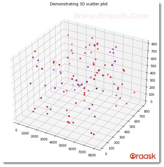
We can plot multiple scatter charts in the three-dimensional figure. We must add multiple scatter3D() functions and pass the variables to the function.

Example (3)

#import all the necessary libraries
import numpy as np
import matplotlib.pyplot as plt

#defining a user-defined function to plot the three-dimensional scatter plot
def three_dimensional_scatter(x1,y1,z1,x2,y2,z2):
    #creating figure object in the plot
    fig = plt.figure(figsize = (9,9))
    #created three-dimensional workspace 
    ax = plt.axes(projection ="3d")
    #plotting the three-dimensional scatter plot using the parameters 
    ax.scatter3D(x1, y1, z1, color = "purple")
    ax.scatter3D(x2, y2, z2, color = "red")
    #defining title to the plot
    plt.title("Demonstrating 3D scatter plot")
    #displaying the three-dimensional scatter plot
    plt.show()
    
#creating the main() function
def main():
    #creating data points for the z-axis
    z1 = np.random.randint(800, size =(50))
    #creating data points for the x-axis
    x1 = np.random.randint(8000, size =(50))
    #creating data points for the y axis
    y1 = np.random.randint(800, size =(50))
    z2 = np.random.randint(800, size =(50))
    #creating data points for the x-axis
    x2 = np.random.randint(8000, size =(50))
    #creating data points for the y-axis
    y2 = np.random.randint(800, size =(50))
    #calling the main() function
    three_dimensional_scatter(x1,y1,z1,x2,y2,z2)

#callng the main() function
if __name__ == "__main__":
    main()

Output:

Plotting Three-Dimensions (3D) With a Color Bar

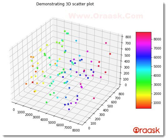
We sometimes need to plot the color bar side by side with the three-dimensional plot. The color bar is used to visualize the relative magnitude of the values of the data points in the plot.

We should understand the following points to plot the color bar in 3D scatter plot.

1. We need to pass a c argument to the scatter3D() function, where we need to set the value to it in terms of x,y, and z. Usually, the standard practice is to use the following value:

c=(x+y+z)

2. We can call an in-built function using the get_cmap() function to get a better color visualization of the plot.
3. We must use the colorbar() function to plot the color bar. There we can pass many other functions like aspect, shrink, etc., to make the color bar more informative.

Example (4)

#import all the necessary libraries
import numpy as np
import matplotlib.pyplot as plt

#defining a user-defined function to plot the three-dimensional scatter plot
def three_dimensional_scatter(x,y,z):
    #creating figure object in the plot
    fig = plt.figure(figsize = (9,9))
    #created three-dimensional workspace 
    ax = plt.axes(projection ="3d")
    my_cmap = plt.get_cmap('hsv')
    #plotting the three-dimensional scatter plot using the parameters 
    scatterplot=ax.scatter3D(x, y, z,cmap = my_cmap,alpha=0.9,c=(x+y+z))
    #defining title to the plot
    plt.title("Demonstrating 3D scatter plot")
    #defining the colorbar in the plot
    fig.colorbar(scatterplot, ax = ax, shrink = 0.5, aspect = 5)
    #displaying the three-dimensional scatter plot
    plt.show()
    
#creating the main() function
def main():
    #creating data points for the z-axis
    z = np.random.randint(800, size =(100))
    print(f"Z values generated are: {z}")
    #creating data points for the x-axis
    x = np.random.randint(8000, size =(100))
    print(f"x values generated are: {x}")
    #creating data points for the y axis
    y = np.random.randint(800, size =(100))
    print(f"y values generated are: {y}")
    #calling the main() function
    three_dimensional_scatter(x,y,z)

#callng the main() function
if __name__ == "__main__":
    main()

Output:

Z values generated are: [679 665 316 534 494  68 174 354 226 140 516 285 245 524 648 270 234  17

 302 142 677 443 277 525 398 247 281 233 250 739 126 456 683 567 700 241

 587 671 159 142  89 358 425 571  52  48 555 511 595 693 765 577  81 142

 130 363 584 144  94 485 424 243 574 309 340 577 309  35 548  78 475 774

 397 605 205 112 482 762 461 151 773  92 247  23 689 393 741 676  87 289

 639 102 437 231 199 384 620 415 149 597]

x values generated are: [7672 1701 3410 7496 7534 6368 5081 1547  960 2121 6381 5877 2929 1217

  996 3297 2646  831 6803 1735 2147 4732 2982 7590  397 5014 4681 5246

 3108 2423 1487 4240 3696 3833 5585  197 7625 6788 5464 3530 3363 6976

 2905 3180 3077 5712  293 6057 2540 1463 2491 1506    7  992 5248 1316

 5440  500 5151 1517 3548  917 2296 6705 7768 5742 3227 3325  491 5842

 4747 2941 3784 1383 7009 7910 5010 6539 1018 6874 6226 6336 4460 1616

 2473 4080 4253 3106 3196 3533 1033 4292 4625  642 6743 5874  893 2005

 6009 3640]

y values generated are: [119  31 389 770  68  26 780 123 753 551 528 501 462 786 327 175 553 203

 232  82 224 348 696 469 249 521 285 231 700 698 291 157 662 200 198 340

 474 799 763 570 211 454  97 170 500 332 235 246  10 790 658 656 295 236

 153  74 322 728 688 716 111 377 300 238 610   6 652  57 249 102 222 471

 729 619 647 312 555 401 258  87 156 218 295 754 182  82 320 171 161 102  462 132 585  66   4 450 335 695   0 249]

Explanation:

1. First, we imported all the necessary libraries and packages in the code using the import statement of python. We imported the numpy and matplotlib.pyplot in the function using their alias names.
2. Next we created the user-defined function named three_dimensional_scatter()  which takes x,y,z as its parameters.Under this function, we first resized the figure using the figsize argument in the figure() function. Next, we created axes for the plot using the axes() function. We set the projection=”3d” to create a three-dimensional plot. Next, we imported cmap using the following lines of codes:

my_cmap = plt.get_cmap(‘hsv’)

3. Next, we plotted the scatter plot in the figure using the scatter3D() function. We first passed the values of x,y, and z. Passing these three values are compulsory in the code. Next, we passed the value of the cmap attribute to my_cmap. We used the alpha attribute, which defines the relative intensity of the data points.0 means no intensity of color, and 1 means maximum intensity. We also passed the c argument and set its value to (x+y+z). We stored these entire statements in some other variable named scatterplot.
4. We now set the title using the title() function. Next, we used the colorbar() function to plot the colorbar in the figure. We passed the scatterplot as one of the arguments. In contrast, the shrink attribute takes a float as an argument. It defines the relative size of the color bar in terms of the axes.aspect attribute defines the height ratio to the color bar’s width.
5. Next, we displayed the plot using the plt.show() function.
6. Next, we created the main() function, which is the main driving code of the program. Under this function, we created the data points for the x,y, and z-axis. We used the numpy library to generate the data points in the code. We also used the string formatting technique and print function to display the generated data points in the code. We called the three_dimensional_scatter() function and passed all the necessary arguments to the plot.
7. Finally, we called the main() function using the following lines of codes:

if __name__ == “__main__”:

    main()

Conclusion

In this article, we have learned how to plot three-dimensional scatter plots in matplotlib python. We have used the scatter3D() function to plot the scatter plot in three dimensions. We also used many other functions and attributed them to making the plots more informative and customizable.

Although we have discussed a lot of functions and attributes in the article, we recommend the readers to please look up the python documentation to get information regarding other associated attributes and functions.