Introduction

The counter graph is a three-dimensional plot in which uniform slices are drawn along the z-axis to create a three-dimensional surface. The link between two independent variables, x and y, and one dependent variable, let’s say z, is plotted using contour graphs. As a result, z depends on x and y. A function with two variables can be precisely identified by using a contour graph.

Contour plots are widely used to plot and visualize different objects and parameters’ density, heights, etc. These plots are extremely useful in engineering, mathematics, science, etc., where there is a need to interpret the density of data points.

This article will explain how to plot the matplotlib contour plots in two and three dimensions and different coordinate systems.

Prerequisite

Before we proceed with the codes, we presume that the reader has sound knowledge of contour plots. We also need some libraries and packages to code. They are namely matplotlib and numpy. In case you haven’t installed them, then perform the following:

If you are a windows user, then open the PowerShell and run the following commands:

pip install matplotlib numpy

If you are a Linux or a macOS user, then open the bash terminal and run the following commands:

pip install matplotlib numpy

How To Plot Contour Plots In Matplotlib

Matplotlib offers us two different functions to plot the contour plots in two and three dimensions. We can also use the same in other coordinate systems like the polar plots.

However, there is some difference in the working between the two functions. While the contour()function will only draw the lines of the plot, the contourf() will both draw the lines as well as fill between the lines. The filling will be based on the density of the data points.

Using the contour() Function

The contour() function of matplotlib allows us to plot the contour plots without filling the region between the lines.

Example (1)

# Import all the necessary libraries and modules in our code
import matplotlib.pyplot as plt
import numpy as np
def contour_plot(X, Y, Z):
    # Creating the figure object
    fig = plt.figure(figsize=(9, 9))
    # Creating the axes object
    ax = plt.axes()
    # Plotting the contour plot
    ax.contour(X, Y, Z)
    # Defining the title of the plot
    ax.set_title('Contour Plot')
    # Defining the label along the x-axis
    ax.set_xlabel('x values')
    # Defining the label along the y axis
    ax.set_ylabel('y values')
    # Displaying the contour plot
    plt.show()
# Creating the main() function
def main():
    # Creating the x-axis value of the data points
    x = np.linspace(-50, 50, 100)
    # Creating the y-axis value of the data points
    y = np.linspace(-50, 50, 100)
    # Creating a 2-D grid of features
    X, Y = np.meshgrid(x, y)
    # Defining the custom function to get the z values
    z = np.power(X, 2)+np.power(Y, 2)
    # Calling the contour() function
    contour_plot(X, Y, z)


# Calling the main() function
if __name__ == "__main__":
    main()

Output:

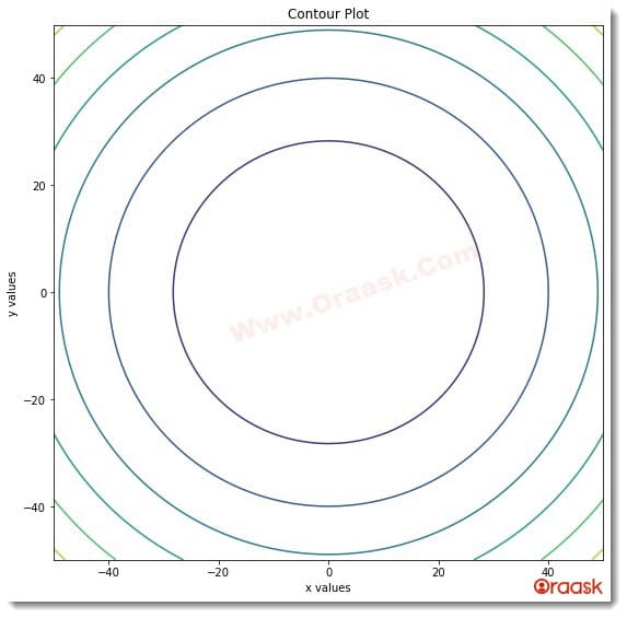
Explanation:

1. First, we imported all the necessary libraries and packages in our code using the import statement of python. We used the technique of aliasing for convenience in writing our code.
2. Next, we used a custom-defined function named contout_plot(). The function is void and takes three arguments, namely X, Y, and Z. Under this function, we first created the figure object using the figure() function of matplotlib. We defined the size of the figure using the figsize attribute of matplotlib. Next, we defined the plot’s axes using the axes() function of matplotlib. Using the function contour(), we plotted the contour plot. We passed the values of X, Y, and Z as the function’s parameters. We set the title for the plot using the set_title() function of matoplotlib. We set the labels along the axes using the set_xlabel() and set_ylabel() functions of matplotlib. Next, we displayed the plot using the plt.show() function. But in Jupyter Notebook, this function is optional to use.
3. Next, we created the main() function, which is the driving code of the program. Under this function, we created data points and took a custom-defined function to plot the function. Note that the X and Y variables are independent, and the variable z is dependent on X and Y. We used the lispace() function of the numpy library to plot the figure. The linspace() function takes three arguments: to start, step, and the number of elements. The start defines the starting number with which the iteration should resume. The stop defines the number up to which the iteration should run. Finally, the last parameter is the number of elements in the array we need to create.
4. After making the data points, however, we need to make a mesh grid out of them to plot the data points in the contour plot.
5. We called the contour_plot() with appropriate arguments to plot the figure.
6. Finally, we called the main() function the driving code with the help of the following lines of codes:

if __name__ == “__main__”:

    main()

Using The Contourf() Function:

The contourf() function, on the other hand, fills the space between the lines.

Example (2)

# Import all the necessary libraries and modules in our code
import matplotlib.pyplot as plt
import numpy as np
def contour_plot(X, Y, Z):
    # Creating the figure object
    fig = plt.figure(figsize=(9, 9))
    # Creating the axes object
    ax = plt.axes()
    # Plotting the contour plot
    ax.contourf(X, Y, Z)
    # Defining the title of the plot
    ax.set_title('Contour Plot using contourf() function')
    # Defining the label along the x-axis
    ax.set_xlabel('x values')
    # Defining the label along the y axis
    ax.set_ylabel('y values')
    # Displaying the contour plot
    plt.show()
# Creating the main() function
def main():
    # Creating the x-axis value of the data points
    x = np.linspace(-30, 30, 100)
    # Creating the y-axis value of the data points
    y = np.linspace(-30, 30, 100)
    # Creating a 2-D grid of features
    X, Y = np.meshgrid(x, y)
    # Defining the custom function to get the z values
    z = np.power(X, 3)+np.power(Y, 5)
    # Calling the contour() function
    contour_plot(X, Y, z)
# Calling the main() function
if __name__ == "__main__":
    main()

Output:

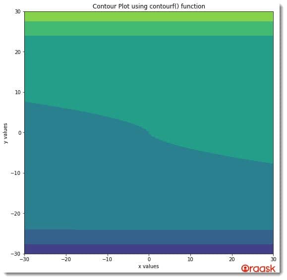
As you can see, there is a difference in the outputs of the contour() and the contourf() functions. While the contour function plots the line, the contourf() function draws the lines and fills the in-between spaces.

Check This: Article on How to Draw a Polar Contour Plot in Matplotlib if you want to know more about how to draw a mix of polar and contour plot in Matplotlib with practical examples.

Plotting Three-Dimensional 3D Contour Plots

Matplotlib also allows us to plot the contour plots in three dimensions too. Here to plot the contour plot in three dimensions, we need first to specify the projection to three dimensions, and next, instead of the contour() and contourf() functions, we need to use the contour3D() functions. To create the three-dimensional contour plot, we must make a mesh grid.

Example (3)

# Import all the necessary modules and functions in the code
import numpy as np
import matplotlib.pyplot as plt
# Create a user-defined function named contour()
def view(x, y, z):
    # Next, create a figure object using the figure () function
    fig = plt.figure(figsize=(9, 9))
    # Creating the figure axes
    ax = plt.axes(projection='3d')
    # Plotting the graph.
    contour_graph = ax.contour3D(x, y, z, 100)
    # Defining the title of the plot
    plt.title("Demonstrating the three dimensional contour plot")
    # Defining the x label
    ax.set_xlabel('x axis')
    # Defining the y label
    ax.set_ylabel('y axis')
    # Defining the z label
    ax.set_zlabel('z axis')
    # Displaying the plot
    plt.show()
# Creating the main () function
def main():
    # Creating data points for the x-axis
    x = np.linspace(-50, 50, 100)
    # Creating data points for the y axis
    y = np.linspace(-50, 50, 100)
    # Creating a mesh grid out of the values of x and y
    x, y = np.meshgrid(x, y)
    # Creating data points for the z-axis
    z = np.power(x, 2)+np.power(y, 2)
    # Calling the contour () function
    view(x, y, z)
# Calling the main() function
if __name__ == "__main__":
    main()

Output:

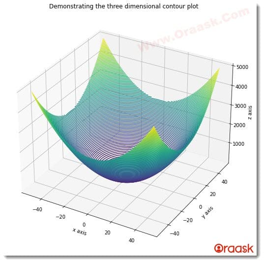
Explanation:

1. We imported the numpy library and the pyplot module in the code using the import statement of python.
2. Next, we created a user-defined function named view(). This is a void function, and it takes three arguments, namely x, y, and z. Under the function, we first defined the figure object using the figure() function of matplotlib. Next, we created the axes object using the axes() function. We specified the projection as ‘3d’ to specify that we wanted a three-dimensional plot. Now we plotted the graph using the contour3D() function. We passed the values of x, y, and z as the parameters for the function and passed another critical parameter, which is a whole number. The number defines the number of slices along the z-axis into which the graph should be cut. We specified the value of this parameter to be 100.
3. Next we specified the labels along the axes with the help of set_xlabel(), set_ylabel() and set_zlabel() functions. We used the plt.show() functions to display the graph.
4. Next, we created the main() function. This is the driving code of the program. Under this function, we created the data points and used the function z=f(x,y)=x^2+y^2 to plot the figure. We called the view() function with appropriate arguments.
5. Finally, we called the main() function with the help of the following lines of codes:

if __name__ == “__main__”:

    main()

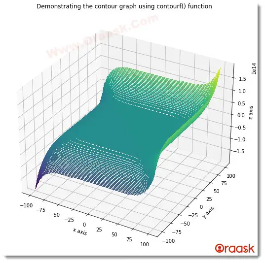
Just like we have created the contour plot using the contour() function, we can also use the contourf() function.

Example (4)

# Import all the necessary modules and functions in the code
import numpy as np
import matplotlib.pyplot as plt
# Create a user-defined function named contour()
def contour(x, y, z):
    # Next, create a figure object using the figure () function
    fig = plt.figure(figsize=(9, 9))
    # Creating the figure axes
    ax = plt.axes(projection='3d')
    # Plotting the graph.
    contour_graph = ax.contourf3D(x, y, z, 100)
    # Defining the x label
    ax.set_xlabel('x axis')
    # Defining the y label
    ax.set_ylabel('y axis')
    # Defining the z label
    ax.set_zlabel('z axis')
    # Defining the title of the plot
    plt.title("Demonstrating the contour graph using contourf() function")
    # Displaying the plot
    plt.show()
# Creating the main () function
def main():
    # Creating data points for the x-axis
    x = np.linspace(-100, 100, 2000)
    # Creating data points for the y axis
    y = np.linspace(-100, 100, 2000)
    x, y = np.meshgrid(x, y)
    # Creating data points for the z-axis
    z = np.power(x, 7)+np.power(y, 7)
    # Calling the contour () function
    contour(x, y, z)
# Calling the main() function
if __name__ == "__main__":
    main()

Output:

Creating A Polar Contour Plot

Matplotlib not only allows us to plot the contour plots in rectangular coordinates, but it also allows us to plot the contour plot in other coordinates, say the polar coordinates. For the polar coordinates, we need to pass the values of the distance of the points from the center of the figure, the angle the line connecting the point and the center of the figure makes, etc.

Example (5)

# Import all the necessary libraries and packages in the code.
import numpy as np
import matplotlib.pyplot as plt
# Creating a user-defined function named contour_plot


def contour_polar(theta, r, values):
    # Creating the figure  object
    fig = plt.figure(figsize=(9, 9))
    # Creating the axes object
    ax = plt.axes(projection="polar")
    # Plotting the first contour plot
    # Plotting the contour plot
    ax.contour(theta, r, values)
    # Defining the title of the plot
    plt.title("Demonstrating polar contour plot")
    # Displaying the contour plot
    plt.show()
# Creating the main() function
def main():
    # Creating data points for the x-axis
    x = np.radians(np.linspace(0, 270, 7))
    # Creating data points for the y axis
    y = np.linspace(0, 270, 7)
    # Creating the mesh grid for plotting the contour plot
    r, theta = np.meshgrid(y, x)
    # Defining the values
    values = np.random.random((7, 7))
    # Printing the x array
    print(f"The x array is: {x}")
    # Printing the y array
    print(f"The y array is: {y}")
    # Printing the r array
    print(f"The r array is: {r}")
    # Printing the theta array
    print(f"The theta array is: {theta}")
    # Prnting the values
    print(values)
    # Calling the contour_plot() function
    contour_polar(theta, r, values)
# Calling the main() function
if __name__ == "__main__":
    main()

Output:

The x array is: [0. 0.78539816 1.57079633 2.35619449 3.14159265 3.92699082
4.71238898]
The y array is: [ 0. 45. 90. 135. 180. 225. 270.]
The r array is: [[ 0. 45. 90. 135. 180. 225. 270.]
[ 0. 45. 90. 135. 180. 225. 270.]
[ 0. 45. 90. 135. 180. 225. 270.]
[ 0. 45. 90. 135. 180. 225. 270.]
[ 0. 45. 90. 135. 180. 225. 270.]
[ 0. 45. 90. 135. 180. 225. 270.]
[ 0. 45. 90. 135. 180. 225. 270.]]
The theta array is: [[0. 0. 0. 0. 0. 0. 0. ]
[0.78539816 0.78539816 0.78539816 0.78539816 0.78539816 0.78539816 0.78539816]
[1.57079633 1.57079633 1.57079633 1.57079633 1.57079633 1.57079633 1.57079633]
[2.35619449 2.35619449 2.35619449 2.35619449 2.35619449 2.35619449 2.35619449]
[3.14159265 3.14159265 3.14159265 3.14159265 3.14159265 3.14159265 3.14159265]
[3.92699082 3.92699082 3.92699082 3.92699082 3.92699082 3.92699082 3.92699082]
[4.71238898 4.71238898 4.71238898 4.71238898 4.71238898 4.71238898 4.71238898]]
[[0.07206057 0.3088822 0.43708635 0.42974978 0.80484263 0.63912403
…
[0.96418781 0.14363606 0.87544587 0.64419877 0.62668948 0.59200001 0.63267986]
[0.37559072 0.55178563 0.07588603 0.66928923 0.32912929 0.44971438 0.80228877]]

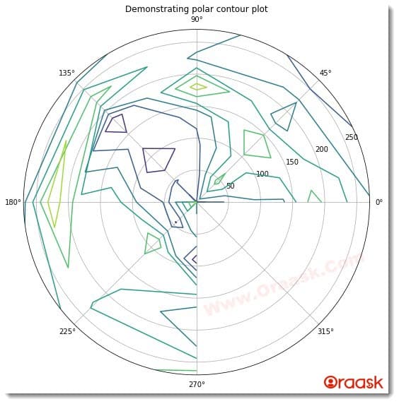
But What Does The Contour Plot Say?

Up to this point, we have learned many ways to create contour plots. We have discussed plotting the contour plots in different dimensions and coordinates too. But still, at this point, you probably did not understand an obvious question- What information do these contour plots display? Before we discuss another question, we would like to address you. Why are we explaining this fundamental question at the end? Well, that’s because to understand the actual message of the contour plot, we need to know the contour plot in two and three dimensions.

Now let us get back to our discussion-What does the contour plot describe? We can answer this by following points:

The contour plot is initially for the three-dimensional plot. This consists of a function dependent on two independent variables, say, x and y. In three dimensions, such plots are known as the contour plot. Let us take one example and understand it throughout

Example (6)

# Import all the necessary libraries and packages in the code
import numpy as np
import matplotlib.pyplot as plt
# Creating a user-defined function called contour
def contour(x, y, z):
    # Creating the figure object
    fig = plt.figure(figsize=(9, 9))
    # Creating the axes object
    ax = plt.axes(projection='3d')
    # Plotting the contour graph
    ax.contour3D(x, y, z, 100)
    # Defining the x label
    ax.set_xlabel('x axis')
    # Defining the y label
    ax.set_ylabel('y axis')
    # Defining the z label
    ax.set_zlabel('z axis')
    # Passing title to the graph
    ax.set_title('Demonstrating contour graph in three dimension')
    # Displaaying the contour graph
    plt.show()
# Creating the main() function
def main():
    # Defining the data point for the x-axis
    x = np.arange(0, 200, 30)
    # Defining the data point for the y axis
    y = np.arange(0, 200, 100)
    # Creating a two-dimensional mesh grid from x and y values
    x, y = np.meshgrid(x, y)
    # Defining the z-axis
    z = np.sin(x)+np.cos(x)
    # Calling the contour function
    contour(x, y, z)
# Calling the main() function
if __name__ == "__main__":
    main()

Output:

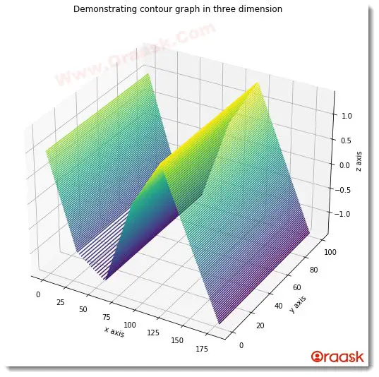
Now this plot actually represents the function z=f(x,y)=sin(x)+cos(x). Yeah, this was that simple!

Two-dimensional contour plot: Now that we have understood what the contour plot describes, let us now look into the two-dimensional contour plot. If you carefully noticed the codes, you should have observed that even the two-dimensional contour plot has another parameter, z. But we know that two dimensions have only two attributes, namely the x and y axes! This is because the two-dimensional plot is a projection of the corresponding three-dimensional figure. Z represents the parent function, and the two-dimensional plot represents the corresponding three-dimensional contour plot projection on the XY plane.

Example (7)

# Import all the necessary libraries and packages in the code
import numpy as np
import matplotlib.pyplot as plt
# Creating a user-defined function called contour
def contour(x, y, z):
    # Creating the figure object
    fig = plt.figure(figsize=(9, 9))
    # Creating the axes object
    ax = plt.axes()
    # Plotting the contour graph
    ax.contour(x, y, z, 100)
    # Defining the x label
    ax.set_xlabel('This is the x axis')
    # Defining the y label
    ax.set_ylabel('This is the y axis')
    # Passing title to the graph
    ax.set_title('Demonstrating contour graph')
    # Displaaying the contour graph
    plt.show()
# Creating the main() function
def main():
    # Defining the data point for the x-axis
    x = np.arange(0, 200, 30)
    # Defining the data point for the y axis
    y = np.arange(0, 200, 100)
    # Creating a two-dimensional mesh grid from x and y values
    x, y = np.meshgrid(x, y)
    # Defining the z-axis
    z = np.sin(x)+np.cos(x)
    # Calling the contour function
    contour(x, y, z)

# Calling the main() function
if __name__ == "__main__":
    main()

Output:

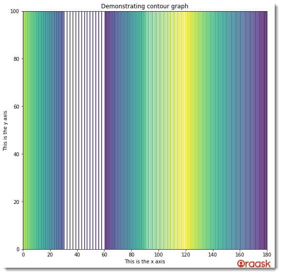
Notice that if you carefully visualize to project the figure of the function z=f(x,y)=sin(x)+cos(x) into the XY place, you will get this graph!

Conclusion

We have discussed plotting the matplotlib contour plots in two and three dimensions. We also discussed how to plot the contour plots in polar coordinates. We used two main functions, namely contour() and contourf() functions, to plot the contour plots. Besides them, we also talked about many of the associated attributes and arguments.

Although we have discussed most of the critical topics, we strongly recommend the readers go through the matplotlib python documentation to understand the topic more.