How Can We Help?
Introduction:
Sometimes the programmers need to fill the regions between two plots. Such plots help visualize optimization problems. One such example is obtaining the optimum value of a particular equation under certain constraints on the values of the variables.
This article will explain how to fill between the lines in matplotlib.
[adinserter block=”1″]
Prerequisite:
Before we jump into the coding part, please ensure that you have the matplotlib and the numpy libraries installed in your system. If you have not done it yet, install the libraries first with the help of the pip package manager.
If you are a windows user, open the PowerShell and if you are a macOS or a Linux user, then open the bash terminal and run the following commands:
pip install numpy matplotlibfill_between function
Matplotlib allows us to fill the region between the lines using many functions and techniques. The most popular technique among them is the fill_between method.
[adinserter block=”2″]
Syntax:
plt.fill_between(\, \, \)The function takes three arguments. However, they are not compulsory. First, two of them are compulsory. If you do not pass the third argument, then python will default plot the space between the plot and the x-axis. Let us take one illustration to understand its usage.
Example (1)
# Import all the necessary libraries and packages in the code
import pylab as plt
import numpy as np
# Creating a user-defined function named fill
def fill(x, y):
    # Creating the figure object
    fig = plt.figure(figsize=(9, 9))
    # Creating the axes object
    ax = plt.axes()
    # Filling between the plots
    ax.fill_between(x, y)
    # Defining the title for the plot
    ax.set_title('fill between y=sin(x) , and y=0')
    # Displaying the plot
    plt.show()
# Creating the main function
def main():
    # Creating the x coordinate for the data points
    x = np.linspace(0, 10, 100)
    # Creating the y coordinate for the data points
    y = np.sin(x)
    # Calling the fill function
    fill(x, y)
# Calling the main function
if __name__ == "__main__":
    main()
Output:
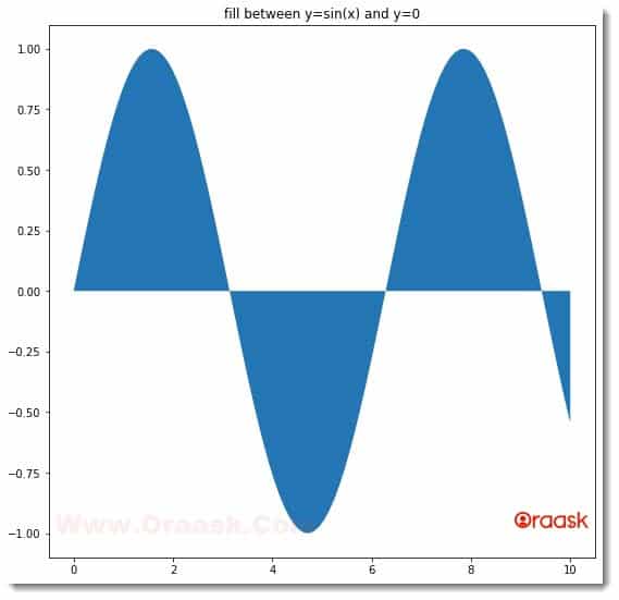
[adinserter block=”3″]
Explanation:
- We first imported necessary libraries and packages in our code using the import statement. We used the technique of aliasing for convenience in writing the codes further.
- Next, we created a user-defined function named fill. The function takes two arguments, called x and y. Under the function, we created the figure object using the figure function of pyplot. We used the axes function to define the axes object. Next, we used the fill_between function to fill between the two plots. Next, we used the set_title function to define the plot’s title. And finally, using the show function, we displayed the plot. Note that we did not use the plot function to plot the two figures. This is not required. We can also use the plot function to plot them; however, the output will remain the same in both cases.
- Next, we created the main function, which is the main driving code of the program. We created all the data points under this function. We used the linspace function of numpy to generate data points. The linspace function takes three basic arguments. They start, stop, and several elements. The start defines the number with which the iteration should start, the stop defines the number up to which the iteration should take place, and the last parameter is self-explanatory.
- We called the fill function with appropriate arguments. Finally, we called the main function using the following lines of codes: if __name__ == “main“: main()
We can perform the same after creating the axes object too. The syntax of the function does not change in such cases. The only difference is that we will be creating the figures through axes.
Example (2)
# Import all the necessary libraries and packages in the code
import matplotlib.pyplot as plt
import numpy as np
# Creating a user-defined function named fill
def fill(x, y):
    # Creating the figure object
    fig = plt.figure(figsize=(9, 9))
    # Creating the axes object
    ax = plt.axes()
    # Filling between the plots
    ax.fill_between(x, y ,color="brown")
    # Defining the title for the plot
    ax.set_title('fill between y=tan(x) , and y=0')
    # Displaying the plot
    plt.show()
# Creating the main function
def main():
    # Creating the x coordinate for the data points
    x = np.linspace(0, 10, 100)
    # Creating the y coordinate for the data points
    y = np.tan(x)
    # Calling the fill function
    fill(x, y)


# Calling the main function
if __name__ == "__main__":
    main()
Output:
[adinserter block=”4″]
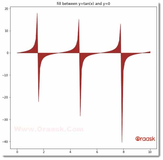
Notice that in the previous two examples, we have passed two arguments only to the function fill_between. We did not pass the third parameter. Python does not complain. Instead, it will simply fill between the graph and the x-axis.
How to Fill Between two Different Line Plots?
Matplotlib also allows us to fill between two different line plots. We need to pass three arguments in such cases.
- The first parameter is the x-axis coordinates of the data points.
- The second parameter is the y coordinates of the data points of the first plot.
- The third parameter is the y coordinates of the data points of the second plot.
[adinserter block=”5″]
Example (3)
# Import all the necessary libraries and packages in the code
import matplotlib.pyplot as plt
import numpy as np
# Creating a user-defined function named fill
def fill(x, y1, y2):
    # Creating the figure object
    fig, (ax1, ax2, ax3) = plt.subplots( 3, 1, sharex=True, figsize=(9, 9))
    # Plotting the first figure
    ax1.plot(x,y1)
    # Defining the title for the first sub-plot
    ax1.set_title('y=sin(x)')
    # Plotting the second figure
    ax2.plot(x,y2)
    # Defining the title for the second sub-plot
    ax3.set_title('y=cos(x)')
    # Filling between the plots
    ax3.fill_between(x, y1, y2 ,color="brown")
    # Defining the title for the third sub-plot
    ax3.set_title('fill between y=tan(x) , and y=0')
    # Displaying the plot
    plt.show()
# Creating the main function
def main():
    # Creating the x coordinate for the data points
    x = np.linspace(0, 10, 100)
    # Creating the y coordinate for the data points of the first plot
    y1 = np.sin(x)
    # Creating the y coordinate for the data points of the second plot
    y2 = np.cos(x)
    # Calling the fill function
    fill(x, y1,y2)
# Calling the main function
if __name__ == "__main__":
    main()
Output:
Explanation:
- We first imported all the necessary libraries and packages to our code using the import statement of python. We used the aliasing names of the libraries.
- Next, we created a user-defined function named fill. The function takes only three parameters: x, y1, and y2.
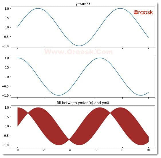
- Under this function, we created the axes and the fig objects. We used the subplot function of python matplotlib to create those objects. We specified 3,1 as the function’s parameters, indicating that we need three rows and only one column of plots in the same workspace. The sharex is the argument which takes bool or {‘none’, ‘all’, ‘row’, ‘col’} as the values. By default, its value is set to False. This defines the sharing of the axes. Here we want all the plots to share the same axes; hence, we set the value of sharex to True.
- Next, we plotted the figure using the plot function. We plotted three different plots in the same figure space to better visualize the effects of the color fill between the lines.
- We set the titles of the plot using the set_title function. Next comes the most critical part. We used the fill_between function to fill between the plots using color. We have passed three parameters, called x, y1, and y2. We used the color argument to set the region’s color between brown lines.
- We used the show function to display the graph.
- Next, we created the main function. This is the driving code of the program. Again, here it is a void function. Under this function, we created the data points for the plots. We used two plots. The first one is for the sine function, and the second one is for the cosine function. We called the fill function with appropriate arguments to plot the figure.
- Finally, we called the main function using the following lines of codes: if __name__ == “main“: main()
Filling With Specific Conditions:
Often, we may not need to fill all the regions between two lines. We may also need to fill only a specific region. Matplotlib allows us to do so with the help of queries. We can use such queries within the function.
[adinserter block=”6″]
Example (4)
# Import all the necessary libraries and packages in the code
import matplotlib.pyplot as plt
import numpy as np
# Creating a user-defined function named fill
def fill(x, y1, y2):
    # Creating the figure object
    fig, (ax1, ax2, ax3, ax4, ax5) = plt.subplots(
        5, 1, sharex=True, figsize=(9, 9))
    # Plotting the first figure
    ax1.plot(x, y1)
    # Defining the title for the first sub-plot
    ax1.set_title('y=sin(x)')
    # Plotting the second figure
    ax2.plot(x, y2)
    # Defining the title for the second sub-plot
    ax2.set_title('y=cos(x)')
    # Filling between the plots
    ax3.fill_between(x, y1, y2, color="yellow")
    # Filling with specific conditions
    ax4.fill_between(x, y1, y2, where=(y1 > y2), color="blue")
    # Defining the title for the fourth sub-plot
    ax4.set_title('Filling regions where the value of sin(x) > cos(x)')
    # Filling with specific conditions
    ax5.fill_between(x, y1, y2, where=(y1 < y2), color="green")
    # Defining the title for the fourth sub-plot
    ax5.set_title('Filling regions where the value of sin(x) < cos(x)')
    # Displaying the plot
    plt.show()
# Creating the main function
def main():
    # Creating the x coordinate for the data points
    x = np.linspace(0, 10, 100)
    # Creating the y coordinate for the data points of the first plot
    y1 = np.sin(x)
    # Creating the y coordinate for the data points of the second plot
    y2 = np.cos(x)
    # Calling the fill function
    fill(x, y1, y2)
# Calling the main function
if __name__ == "__main__":
    main()
Output:
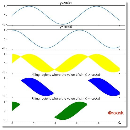
In the above code, we only used an extra parameter: the query. We used the following statements:
- ax4.fill_between(x, y1, y2, where=(y1 > y2), color=”blue”): The statements define that we only need to have those regions filled where the value of y1 (sine function) is greater than the value of y2 (cosine function).
- ax5.fill_between(x, y1, y2, where=(y1 \< y2), color=”green”): The statements define that we only need to have those regions filled where the value of y1 (sine function) is lesser than the value of y2 (cosine function).
[adinserter block=”7″]
Interpolation:
Until now, the examples we have seen mainly consisted of continuous data where we did not see any dramatic change in the values. However, we often encounter situations where one of the plots gains a very high value over the other. In such cases, the matplotlib will not interpolate all the regions between them. This scenario is more specific for the plots where the values are discontinuous. In such a scenario, we need to use the interpolation method of the matplotlib fill_between function.
Example (5)
# Import all the necessary libraries and packages in the code
import matplotlib.pyplot as plt
import numpy as np
# Creating a user-defined function named fill
def fill(x, y1, y2):
    # Creating the figure object
    fig, (ax1, ax2) = plt.subplots(2, 1, sharex=True, figsize=(9, 9))
    # Plotting the first figure
    ax1.plot(x, y1)
    ax1.plot(x, y2)
    # Filling between the regions without interpolation
    ax1.fill_between(x, y1, y2, where=(y1 > y2), color='green', alpha=0.5)
    ax1.fill_between(x, y1, y2, where=(y1 < y2), color='red', alpha=0.5)
    # Defining the title for the first sub-plot
    ax1.set_title('First plot')
    # Plotting the second figure
    ax2.plot(x, y1)
    ax2.plot(x, y2)
    # Filling between the regions with interpolation
    ax2.fill_between(x, y1, y2, where=(y1 > y2),
                     color='green', alpha=0.5, interpolate=True)
    ax2.fill_between(x, y1, y2, where=(y1 <= y2),
                     color='red', alpha=0.5, interpolate=True)
    # Defining the title for the second sub-plot
    ax2.set_title('Second plot')
    # Displaying the plot
    plt.show()
# Creating the main function
def main():
    # Creating the x coordinate for the data points
    x = np.linspace(1, 10, 10)
    # Creating the y coordinate for the data points of the first plot
    y1 = np.array([0.8, 0.8, 0.6, 0.6, 0.6, 0.2, 0.2, 0.2, 0.2, 0.2])
    # Creating the y coordinate for the data points of the second plot
    y2 = np.array([0.2, 0.2, 0.2, 0.2, 0.2, 0.8, 0.8, 0.6, 0.6, 0.6])
    # Calling the fill function
    fill(x, y1, y2)
# Calling the main function
if __name__ == "__main__":
    main()
Output:
[adinserter block=”8″]
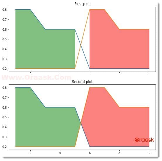
In the above figure, notice that for the first figure, matplotlib did not perform the interpolation by default. However, in the second plot, we passed True as the value for the interpolation; hence, matplotlib did the interpolation for us.
Another parameter we passed to the function is the alpha. We use this function to set the opacity of the color between the plots. The function takes a float as the value. The values should be between 0 and 1. 0 defines no opacity, and 1 defines the maximum opacity.
Using The imshow Function
Matplotlib also allows us to fill between the plots through the imshow function. We need to pass the constraint values. Python automatically fills the values between the plots.
Example (6)
# Import all the necessary libraries and packages in the code
import matplotlib.pyplot as plt
import numpy as np
# Creating a user-defined function named fill
def fill(x,d,y,cos_val,sin_val):
    # Creating the figure object
    fig = plt.figure(figsize=(9, 9))
    # Filling between the plots
    plt.imshow(((y>cos_val) & (y<sin_val) ), extent=(x.min(),x.max(),y.min(),y.max()),origin="lower", cmap="Blues", alpha = 0.3)
    plt.title('fill between y=sin(x) and y=cos(x) with constraints')
    # Displaying the plot
    plt.show()
# Creating the main function
def main():
    # Creating the x coordinate for the data points
    d = np.linspace(-2,10,3000)
    # Creating the meshgrid
    x,y = np.meshgrid(d,d)
    # Creating the cosine value
    cos_val=np.cos(d)
    # Creating the sine value
    sin_val=np.sin(d)
    # Calling the fill function
    fill(x,d, y,cos_val,sin_val)
# Calling the main function
if __name__ == "__main__":
    main()
Output:
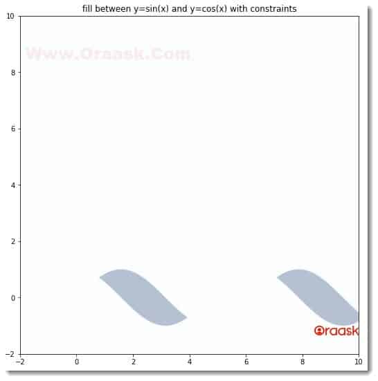
Visualizing linear programming through matplotlib
This section illustrates the applications of filling the region between the line plots in matplotlib.
[adinserter block=”9″]
Problem:
Calculate the maximal and minimal value of z = 5x + 3y for the following constraints.
x + 2y ≤ 14
3x – y ≥ 0
x – y ≤ 2
We only need to plot and get the lines’ intersections in such a problem. One of the intersecting points gives the value of x and y coordinates for which the value of z will be maximum.
Although our aim in this section is not to find the optimum value but to plot the region and visualize the intersecting points, which can give us the optimized value for z.
Example (7)
[adinserter block=”10″]
# Import all the necessary libraries and packages in the code
import matplotlib.pyplot as plt
import numpy as np
# Creating a user-defined function named fill
def fill(x, d, y, y1, y2, y3):
    # Creating the figure object
    fig = plt.figure(figsize=(9, 9))
    # Plotting the line y1 = (14-d)/2
    plt.plot(d, y1)
    # Plotting the line y2=(3*d)
    plt.plot(d, y2)
    # Plotting the line y3=(d-2)
    plt.plot(d, y3)
    # Filling between the plots
    plt.imshow(((x + 2*y <= 14) & (3*x - y >= 0) & (x - y <= 2)).astype(int),
               extent=(x.min(), x.max(), y.min(), y.max()), origin="lower", cmap="Greys", alpha=0.3)
    plt.title('Vislaizing linear programming problem through matplotlib')
    # Displaying the plot
    plt.show()
# Creating the main function
def main():
    # Creating the x coordinate for the data points
    d = np.linspace(-10, 10, 3000)
    # Creating the meshgrid
    x, y = np.meshgrid(d, d)
    y1 = (14-d)/2
    y2 = (3*d)
    y3 = (d-2)
    # Calling the fill function
    fill(x, d, y, y1, y2, y3)
# Calling the main function
if __name__ == "__main__":
    main()
Output:
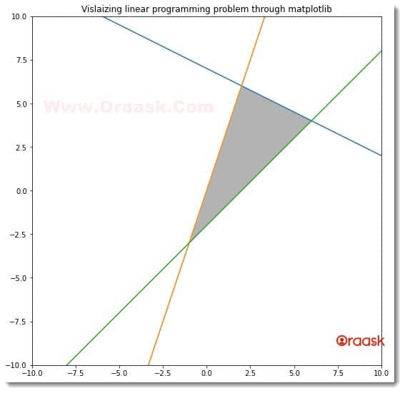
We got three nodes, and the answer comes from any of these three nodes. We only need to find the nodes’ corresponding (x,y) pairs and put them in the equation z= z = 5x + 3y. Our answer would be the pair with the maximum value of z.
Conclusion:
In this article, we have discussed how to fill between the line plots in matplotlib. We have used the fill_between function to fill between the lines. We can use this function in everyday usage and with the axes objects. We can also change the opacity of the color in between. We use the interpolate attribute to fill all the regions by interpolation. We can also select regions between the lines where we need to fill the colors using the queries.
Although we learned most of the important stuff in this article, we strongly recommend that the readers go through the official documentation of matplotlib and explore more about the functions and the attributes.


