The counter graph is a three-dimensional plot in which uniform slices are drawn along the z-axis to create a three-dimensional surface. The link between two independent variables, x and y, and one dependent variable, let’s say z, is plotted using contour graphs. As a result, z depends on x and y. A function with two variables can be precisely identified by using a contour graph.

This article will explain how to plot a polar contour plot.

Prerequisite:

Before we start the coding part, we expect the readers to know the polar plots and the contour plot well.

We need to have the matplotlib and numpy library installed on our machine. If you have not installed them yet, then open the PowerShell if you are a windows user or bash terminal if you are a macOS or Linux user and run the following command:

Pip install matplotlib numpy

How To Plot A Polar Contour Plot?

There are two functions available in matplotlib to plot the contour plot. They are the contour() and contourf() functions. There is, however, a difference between the two functions. The contour() function will only draw the lines, but the contourf() will draw the lines and fill the region between them. Surprisingly the contourf() function is more widely used.

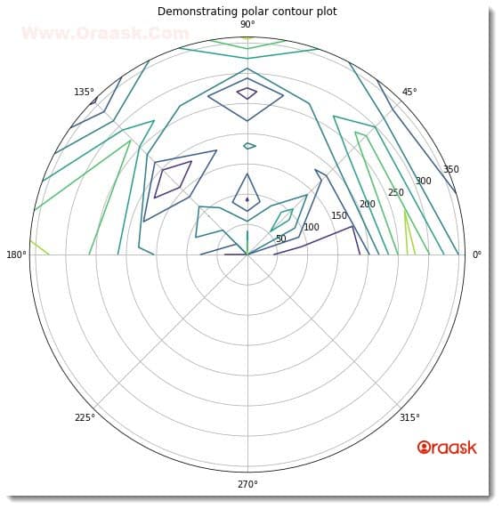
The following code illustrates the use of the contour() function to plot a polar contour graph.

Example (1)

# Import all the necessary libraries and packages in the code.
import numpy as np
import matplotlib.pyplot as plt
# Creating a user-defined function named contour_plot
def contour_polar(theta, r, values):
    # Creating the figure  object
    fig = plt.figure(figsize=(9, 9))
    # Creating the axes object
    ax = plt.axes(projection="polar")
    # Plotting the first contour plot
    # Plotting the contour plot
    ax.contour(theta, r, values)
    # Defining the title of the plot
    plt.title("Demonstrating polar contour plot")
    # Displaying the contour plot
    plt.show()
# Creating the main() function
def main():
    # Creating data points for the x-axis
    x = np.radians(np.linspace(0, 180, 5))
    # Creating data points for the y axis
    y = np.linspace(0, 360, 5)
    # Creating the mesh grid for plotting the contour plot
    r, theta = np.meshgrid(y, x)
    # Defining the values
    values = np.random.random((5, 5))
    # Printing the x array
    print(f"The x array is: {x}")
    # Printing the y array
    print(f"The y array is: {y}")
    # Printing the r array
    print(f"The r array is: {r}")
    # Printing the theta array
    print(f"The theta array is: {theta}")
    # Prnting the values
    print(values)
    # Calling the contour_plot() function
    contour_polar(theta, r, values)


# Calling the main() function
if __name__ == "__main__":
    main()

Output:

The x array is: [0. 0.78539816 1.57079633 2.35619449 3.14159265]

The y array is: [ 0. 90. 180. 270. 360.]

The r array is: [[ 0. 90. 180. 270. 360.]

[ 0. 90. 180. 270. 360.]

[ 0. 90. 180. 270. 360.]

[ 0. 90. 180. 270. 360.]

[ 0. 90. 180. 270. 360.]]

The theta array is: [[0. 0. 0. 0. 0. ]

[0.78539816 0.78539816 0.78539816 0.78539816 0.78539816]

[1.57079633 1.57079633 1.57079633 1.57079633 1.57079633]

[2.35619449 2.35619449 2.35619449 2.35619449 2.35619449]

[3.14159265 3.14159265 3.14159265 3.14159265 3.14159265]]

[[2.59989198e-01 3.10873146e-02 8.86928116e-02 9.48668477e-01

3.83442176e-01]

[4.85727794e-01 6.76238766e-01 2.70950742e-01 8.08790086e-01

1.53375415e-01]

[9.45183913e-01 1.36880978e-01 4.69752545e-01 9.67174884e-02

9.29983736e-01]

[1.85077999e-01 6.01083784e-01 2.54322424e-04 7.49669207e-01

1.23020368e-01]

[7.94254434e-03 3.44985227e-01 4.92396721e-01 7.76191982e-01

9.69992844e-01]]

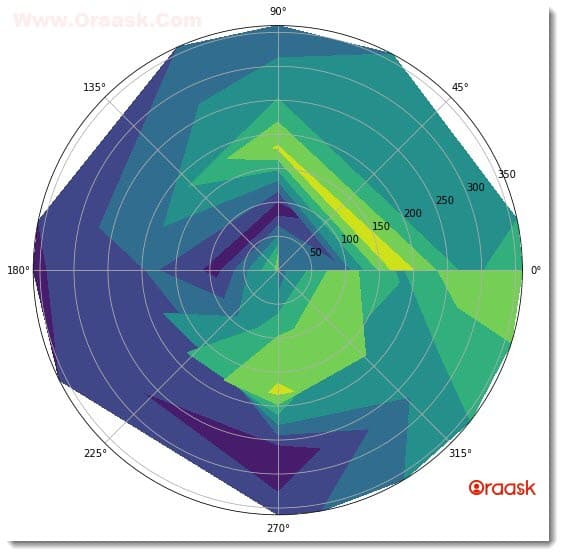
The following code illustrates the use of the contourf() function to plot a polar contour plot.

Example (2)

# Import all the necessary libraries and packages in the code.
import numpy as np
import matplotlib.pyplot as plt
# Creating a user-defined function named contour_plot
def contour_polar(theta, r, values):
    # Creating the figure and axes object
    fig, ax = plt.subplots(subplot_kw=dict(projection='polar'), figsize=(9, 9))
    # Plotting the contour plot
    ax.contourf(theta, r, values)
    # Displaying the contour plot
    plt.show()
# Creating the main() function
def main():
    # Creating data points for the x-axis
    x = np.radians(np.linspace(0, 360, 5))
    # Creating data points for the y axis
    y = np.linspace(0, 360, 5)
    # Creating the mesh grid for plotting the contour plot
    r, theta = np.meshgrid(y, x)
    # Defining the values
    values = np.random.random((5, 5))
    # Printing the x array
    print(f"The x array is: {x}")
    # Printing the y array
    print(f"The y array is: {y}")
    # Printing the r array
    print(f"The r array is: {r}")
    # Printing the theta array
    print(f"The theta array is: {theta}")
    # Prnting the values
    print(values)
    # Calling the contour_plot() function
    contour_polar(theta, r, values)
# Calling the main() function
if __name__ == "__main__":
    main()

Output:

The x array is: [0. 1.57079633 3.14159265 4.71238898 6.28318531]

The y array is: [ 0. 90. 180. 270. 360.]

The r array is: [[ 0. 90. 180. 270. 360.]

[ 0. 90. 180. 270. 360.]

[ 0. 90. 180. 270. 360.]

[ 0. 90. 180. 270. 360.]

[ 0. 90. 180. 270. 360.]]

The theta array is: [[0. 0. 0. 0. 0. ]

[1.57079633 1.57079633 1.57079633 1.57079633 1.57079633]

[3.14159265 3.14159265 3.14159265 3.14159265 3.14159265]

[4.71238898 4.71238898 4.71238898 4.71238898 4.71238898]

[6.28318531 6.28318531 6.28318531 6.28318531 6.28318531]]

[[0.37504905 0.31696578 0.99275336 0.57923922 0.63553504]

[0.9672334 0.04302605 0.91443787 0.52424932 0.3667207 ]

[0.78232707 0.09755662 0.3077626 0.26025732 0.11815233]

[0.2534237 0.73296948 0.92887958 0.01882718 0.22535225]

[0.38379547 0.83021589 0.57769742 0.85787386 0.87473257]]

Explanation:

1. First, we imported the necessary libraries and packages in our code using the import statement of python. We used the technique of aliasing names to write the codes in our program conveniently.
2. Next we created a user-defined function named contour_plot(). The function is void and takes three parameters: theta, r, and values. Under this function, we first created the figure, and the axes object using the subplots() function. We used the attribute projection=” polar” to specify that we want to plot polar coordinates.
3. We plotted the contour plot using the contourf() function. We passed the value of theta, r, and values to this function.
4. We used the plt.show() function to display the graph. Note that this is optional in Jupyter Notebook, and we can safely skip this step.
5. Next, we created the main() function, which is the driving code of the program. Under this function, we created all the data points required for plotting the graph. We used the radians() function of numpy to convert the degree values into radians values. We used the lispace function to generate the data points. The linspace function takes three parameters: to start, stop, and the number of elements. The start defines the number with which the iteration should start in the code. The stop defines the number up to which the iteration should run, and the last parameter defines the total number of elements required.
6. We took 0 as the first and 360 as the last elements to get the values in degree and converted them into radians values using the np.radians() function of numpy. Next, we created a mesh grid out of y and x. This is a crucial step to map the data points correctly in the plot.
7. We also created the values array and used the random.the random() function of the numpy library. We printed all the values of x, y, r, and theta to understand the plot better.
8. We called the contour_polar() function with appropriate arguments there, r, and values.
9. Finally, we called the main() function with the help of the following lines of codes: if __name__ == “main“: main()

Check This: I have wrote a full guide on Matplotlib Contour Plot if you want to know more about contour plot in python matplotlib library (What it is and how to plot a contour plot using different functions and techniques).

How to Plot Multiple Contour Plots

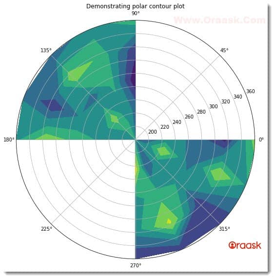
Plotting multiple contour plots in the exact figure is quite an easy task. As we have seen for other plots, we need to call the contour() function multiple times to plot multiple plots in the figure. We can use all the other attributes associated with the function.

Example (3)

# Import all the necessary libraries and packages in the code.
import numpy as np
import matplotlib.pyplot as plt
# Creating a user-defined function named contour_plot
def contour_polar(theta1, r1, theta2, r2, values1, values2):
    # Creating the figure  object
    fig = plt.figure(figsize=(9, 9))
    # Creating the axes object
    ax = plt.axes(projection="polar")
    # Plotting the first contour plot
    ax.contourf(theta1, r1, values1)
    # Plotting the second contour plot
    ax.contourf(theta2, r2, values2)
    # Defining the title of the plot
    plt.title("Demonstrating polar contour plot")
    # Displaying the contour plot
    plt.show()
# Creating the main() function
def main():
    # Creating data points for the x-axis
    x1 = np.radians(np.linspace(90, 180, 5))
    x2 = np.radians(np.linspace(270, 360, 5))
    # Creating data points for the y axis
    y = np.linspace(180, 360, 5)
    # Creating the mesh grid for plotting the contour plot
    r1, theta1 = np.meshgrid(y, x1)
    r2, theta2 = np.meshgrid(y, x2)
    # Defining the values
    values1 = np.random.random((5, 5))
    values2 = np.random.random((5, 5))
    # Printing the x1 array
    print(f"The x array is: {x1}")
    # Printing the x2 array
    print(f"The x array is: {x2}")
    # Printing the y array
    print(f"The y array is: {y}")
    # Printing the r1 array
    print(f"The r array is: {r1}")
    # Printing the r2 array
    print(f"The r array is: {r2}")
    # Printing the theta array
    print(f"The theta array is: {theta1}")
    # Prnting the values1 array
    print(f"The values array is: {values1}")
    # Prnting the values2 array
    print(f"The values array is: {values2}")
    # Calling the contour_plot() function
    contour_polar(theta1, r1, theta2, r2, values1, values2)
# Calling the main() function
if __name__ == "__main__":
    main()

Output:

The x array is: [1.57079633 1.96349541 2.35619449 2.74889357 3.14159265]

The x array is: [4.71238898 5.10508806 5.49778714 5.89048623 6.28318531]

The y array is: [180. 225. 270. 315. 360.]

The r array is: [[180. 225. 270. 315. 360.]

[180. 225. 270. 315. 360.]

[180. 225. 270. 315. 360.]

[180. 225. 270. 315. 360.]

[180. 225. 270. 315. 360.]]

The r array is: [[180. 225. 270. 315. 360.]

[180. 225. 270. 315. 360.]

[180. 225. 270. 315. 360.]

[180. 225. 270. 315. 360.]

[180. 225. 270. 315. 360.]]

The theta array is: [[1.57079633 1.57079633 1.57079633 1.57079633 1.57079633]

[1.96349541 1.96349541 1.96349541 1.96349541 1.96349541]

[2.35619449 2.35619449 2.35619449 2.35619449 2.35619449]

[2.74889357 2.74889357 2.74889357 2.74889357 2.74889357]

[3.14159265 3.14159265 3.14159265 3.14159265 3.14159265]]

The values array is: [[0.39906146 0.42801889 0.00596524 0.17761672 0.67730135]

[0.77051309 0.50355746 0.63658259 0.7104146 0.54039025]

[0.43507246 0.83161953 0.37668466 0.85522391 0.31230775]

[0.40899151 0.58989089 0.46224355 0.17194833 0.43110526]

[0.95178118 0.54466784 0.68865241 0.85905055 0.55502798]]

The values array is: [[0.53871043 0.98513685 0.5498829 0.53249386 0.16841864]

[0.41404275 0.28421747 0.67874045 0.93206074 0.16727791]

[0.52960038 0.56098104 0.58651653 0.19751675 0.16720288]

[0.21657442 0.89095393 0.35605254 0.89310824 0.57696541]

[0.18915657 0.50619404 0.42379593 0.09479061 0.81739328]]

Explanation:

1. First, we imported the numpy library and the matplotlib.pyplot module in our code using the import statement of python.
2. Next we created the contour_plot() function. The function is again a void function, and it takes 6 parameters, called theta1, r1, theta2, r2, values1, and values2. Under the function, we first created the figure object using the plt.figure() function. We specified the plot’s size using the function’s figsize attribute. Next, we created the axes objected using the axes() function and specified the projection of the plot to “polar”. We used the contourf() function of matplotlib to plot the figures. We plotted two different figures and called the function twice with appropriate parameters. Next, we defined the plot’s title using the title() function of matplotlib. We used the show() function to display the plot.
3. After the contour_polar() function we created the main() function. The main() function is the driving code of the program. The interpreter will first search for this function in the entire program and run it first. Under this function, we created the data points for the axes. We used two different variables, x1 and x2, to plot two different plots in the figure.
4. We created the array for the y variable and used the meshgrid() function to create a mesh grid out of the variables y,x1, and y,x2. We printed all the values we created to understand the plot better.
5. We called the contour_polar() function and finally called the main() function.

Plotting Polar Contour Plot Of Fetched Data Set

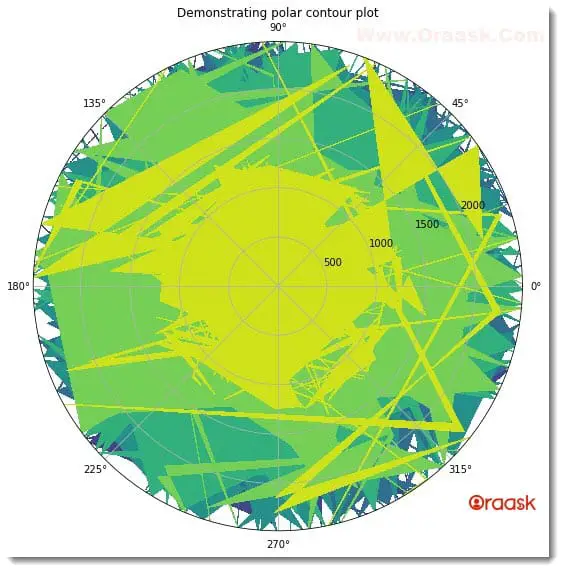
We have used custom-defined datasets to plot the polar contour plots. However, we will not be making custom data sets in real life. Instead, we will fetch the datasets from the CSV of the excel files available. In this section, we will learn how to plot contour plots after fetching the data sets from the CSV or excel files.

Example (4)

# Import all the necessary libraries and packages in the code.
import numpy as np
import matplotlib.pyplot as plt
import pandas as pd
# Creating a user-defined function named contour_plot
def contour_polar(theta, r, values):
    # Creating the figure  object
    fig = plt.figure(figsize=(9, 9))
    # Creating the axes object
    ax = plt.axes(projection="polar")
    # Plotting the contour plot
    ax.contourf(theta, r, values)
    plt.title("Demonstrating polar contour plot")
    # Displaying the contour plot
    plt.show()
# Creating the main() function
def main():
    # Creating data points for the x-axis
    data = pd.read_csv("Housing.csv")
    # Creating the data frame
    df = pd.DataFrame(data)
    # Creating data points for the x array
    x = df["total_rooms"]
    # Creating data points for the y array
    y = df["total_bedrooms"]
    # Creating the meshgrid for plotting the contour plot
    r, theta = np.meshgrid(y[:100], x[:100])
    # Defining the values
    values = np.random.random((100, 100))
    # Printing the x array
    print(f"The x array is: {x}")
    # Printing the y array
    print(f"The y array is: {y}")
    # Printing the r array
    print(f"The r array is: {r}")
    # Printing the theta array
    print(f"The theta array is: {theta}")
    # Prnting the values
    print(f"The values array is: {values}")
    # Calling the contour_plot() function
    contour_polar(theta, r, values)
# Calling the main() function
if __name__ == "__main__":
    main()

Output:

The x array is: 0 880.0

1 7099.0

2 1467.0

3 1274.0

4 1627.0

…

20635 1665.0

20636 697.0

20637 2254.0

20638 1860.0

20639 2785.0

Name: total_rooms, Length: 20640, dtype: float64

The y array is: 0 129.0

1 1106.0

2 190.0

3 235.0

4 280.0

…

20635 374.0

20636 150.0

20637 485.0

20638 409.0

20639 616.0

Name: total_bedrooms, Length: 20640, dtype: float64

The r array is: [[ 129. 1106. 190. … 107. 1270. 1085.]

…

…

[0.67547611 0.14181543 0.59255215 … 0.28677161 0.59923677 0.78444828]

[0.21973213 0.78595105 0.68913415 … 0.86896261 0.58959272 0.4418207 ]

[0.15267056 0.94730901 0.42527655 … 0.37673363 0.66966163 0.85114611]]

Explanation:

1. We first imported the libraries in the code. We imported the numpy and the pandas library, and the matplotlib.pyplot module in the code.
2. Next we created a user-defined function named contour_plot() function. The function is void and takes three parameters: theta, r, and values. Under this function, we first created the figure and the axes object. We specified the size of the figure using the figsize attribute of the function.
3. We used the code’s contourf() function with appropriate parameters to plot the graph. Using the title function, we defined the title of the plot.
4. We create the main() function afterward. Under the main() function. Under this function, we first imported the dataset using the read_csv() function of the pandas library. Next, we created the data frame using the DataFrame() function. We created a meshgrid out of the x and y array.
5. We printed all the arrays for a better understanding of the plot. We called the contour_polar() function with appropriate arguments.
6. Finally, we called the main() function using the following lines of code:

if __name__ == “main“:

main()

Conclusion

In this article, we have learned how to use the contour() and contourf() functions to plot contour plots in matplotlib. Both of them are pretty different from each other in terms of displaying the graph. The contour() function only displays the lines without filling the color between them. The contourf() function, however, both plots the lines and fills the regions in between.

We have learned about the associated attributes and functions. However, we strongly recommend that readers look up the python matplotlib documentation for more information about the associated attributes and functions.