Cubes are famous figures in the field of mensuration/measurement of mathematics. The cube is a three-dimensional figure. Also, they have 12 edges, 6 sides, and 8 corners in total.

This article will explain how to plot the three-dimensional cubes in the matplotlib.

Prerequisite:

We need to install a few of the libraries of python. We need matplotlib, numpy, and mpl_toolkits to plot the upcoming figures.

To install those libraries, we need to type the following lines in PowerShell of windows and bash terminal of the Linux of macOS:

pip install matplotlib
pip install numpy
pip install mpl_toolkits.clifford

Plot Simple Solid Cubes in Three Dimensions (3D)

Plotting solid cubes in the three dimensions can be done with the matplotlib and mpl_toolkits library. We use the voxels() function to plot the cubes in three dimensions. However, plotting the cubes using the functions is not straightforward because we need to define a couple of other functions, attributes, and techniques to implement the cubes in three dimensions. For example, to plot the cubes, we need to define the sides of the cube, The color or the color codes for the face, the dimensions of the axes, etc.

Example (1)

# Import all the necessary libraries in the code
import matplotlib.pyplot as plt
from mpl_toolkits.mplot3d import Axes3D
import numpy as np
# Defining a custom-defined function cubes
def cubes(sides):
    # Creating data points for the sides
    data = np.ones(sides)
    # Creating the figure object
    fig = plt.figure(figsize=(9, 9))
    # Creating axes object to the plot
    ax = fig.add_subplot(111 , projection = '3d')
    # Plotting the figure
    ax.voxels(data, facecolors="yellow")
    # Displaying the figure
    plt.show()
# Creating the main () function
def main():
    # Defining side for the cube
    sides = np.array([ 2, 2, 2 ])
    # Calling the cubes () function
    cubes(sides)
# Calling the main () function
if __name__ == "__main__":
    main ()

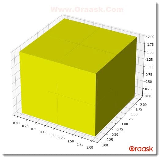
Output:

Explanations:

1. First, we imported all the necessary libraries and packages into our code using the python import statement. We used the alias names of the libraries for convenience.
2. Next, we have created a user-defined function named cubes which takes only one argument, namely sides. Under this function, we first created a variable named data which we used to store the dimension of the cubes. Next, we created a figure object and specified the size of the figure using the attribute named figsize. Next, we created the axes object in the function using the add_subplots () function and specified the projection to “3d”. Next, we plotted the graph using the voxel () function and passed the data as the function’s parameter. We have set another attribute named facecolors which defines the colors of the faces of the cube. We specified it to be yellow.
3. Next, we displayed the plot using the plt.show() function and created the main() function. The main() function is the main driving code of the program. Under this function, we first created the data points for the sides of the cubes using the numpy library. We have used the array () function to create the data points. We called the cubes() function.
4. Finally, we called the main () ( function using the following lines of codes:

if __name__ == “__main__”:

    main ()

Creating Cubes with Different Color Grids

Sometimes we may need to plot cubes with different color grids compared to all the grids with a single color. We can find such a kind of design in the Rubrics cubes. Matplotlib allows us to achieve the same through the usage of a few functions. We should first create the colors for the grids using the np.empty() function.

This will generate matrices with random numbers within. Then we need to define the color of each of the grids. We can either use string to specify the color or the RGB color codes to specify the colors of the grids. We should also set the contrast of the colors using the alpha attribute. Note that we can specify the colors through color codes in the form of numbers. For example, [0, 0, 1, alpha] at alpha=0.9 represents the color of the grid to be blue and the contrast to be 90% of the actual color contrast of the monitor.

Check This: There is a full guide on Matplotlib 3D Bar Chart if you want to know more about 3D Charts.

Example (2)

# Import all the necessary libraries and modules in the code
import matplotlib.pyplot as plt
from mpl_toolkits.mplot3d import Axes3D
import numpy as np
# Defining a custom-defined function cube
def cubes(sides):
    # Creating data points for the sides
    data = np.ones(sides ,  dtype = bool)
    # Defining the transparency of the colors for the cubes
    alpha = 0.9
    # Defining data points for the color of the sides
    colors = np.empty(axes + [4], dtype=float)
    # Defining the color of each grid
    colors[0] = [1 , 0 , 1 , alpha]
    colors[1] = [0 , 1 , 0, alpha]
    colors[2] = [0 , 1 , 1 , alpha]
    colors[3] = [1 , 1 , 0 , alpha]
    colors[4] = [0 , 0 , 1 , alpha]
    # Creating the figure object
    fig = plt.figure(figsize= ( 9,  9 ))
    # Creating the axes object
    ax = fig.add_subplot(111 , projection = '3d')
    # Plotting the graph
    ax.voxels(data, facecolors=colors, edgecolors = 'white')
    # Defining the title of the plot
    plt.title("Demonstrating three dimensional cubes")
# Defining the main() function
def main():
    # Defining the side of the cube
    sides = [5, 5, 5]
    # Calling the cubes () function
    cubes(sides)
# Calling the main () function
if __name__ == "__main__":
    main ()

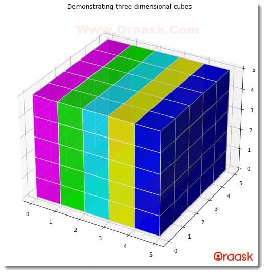
Output:

Explanation:

1. First, as customary, we have imported all the necessary libraries and packages in our code using the import statement of python. We have imported the libraries using their alias names.
2. Next, we created the cubes () function, a user-defined function that takes only one argument. Under this function, we first created the variable data to generate the sides of the cube. Next, we created another variable, alpha which defines the transparency of the colors. The alpha value should be between 0 and 1.0 means there is 0 intensity, and 1 means maximum intensity.
3. After that, we created the colors variable, which will create matrices to store the RGB values of the colors we specify for each grid. We have specified the data type of the values to be float. Next, we set the colors to the grids using the RGB values, and we also passed the alpha parameter to specify the contrast of the colors used.
4. Next, we created the figure object using the plt.figure() function and set the size of the figure using the figsize attribute. Now we have used the add_subplot() function to create the axes object. Next, we plotted the graph using the voxel () function. We have passed the data as the first parameter. This is the mandatory parameter for the function. We also set face colors to the plots using the facecolors attribute and passed colors as the value o this attribute. We then set the title to the plot using the title () function.
5. Next, we created the main () function. Under this function, we defined the sides of the cube. We then called the cubes () function and passed the sides argument to the function.
6. Finally, we called the main () function using the following lines of codes:

if __name__ == “__main__”:

    main ()

Generating Cubes Through Voxels

We can also use other functions and techniques to plot three-dimensional cubes in the plot. One such function is the voxelarray () function. For generating cubes using this function, we first need to define the size of the axes. We can do this with the help of the np.indices() function. Or we can employ any other list-like objects to create the size of the axes. Next, we can define the color of the cubes through the voxelarray object. We can then plot the figure with the help of the voxels () function.

Example (3)

# Import all the necessary libraries and packages in the code
import matplotlib.pyplot as plt
import numpy as np
# Defining the user-defined cubes() function
def cubes(side):
    # Defining the size of the axes
    x, y, z = np.indices((10, 10, 10))
    # Defining the length of the sides of the cubes
    cube = (x < side) & (y < side) & (z < side)
    # Defining the shape of the figure to be a cube
    voxelarray = cube
    # Defining the colors for the cubes
    colors = np.empty(voxelarray.shape, dtype=object)
    # Defining the color of the cube
    colors[cube] = 'purple'
    # Defining the axes and the figure object
    ax = plt.figure(figsize=(9, 9)).add_subplot(projection='3d')
    # Plotting the cube in the figure
    ax.voxels(voxelarray , facecolors=colors, edgecolor='k')
    # Defining the title of the graph
    plt.title("Three dimensional cubes")
    # Displaying the graph
    plt.show()
# Defining the main() function
def main():
    # Defining the side of the cube
    sides = 7
    # Calling the cubes () function
    cubes(sides)
# Calling the main () function
if __name__ == "__main__":
    main ()

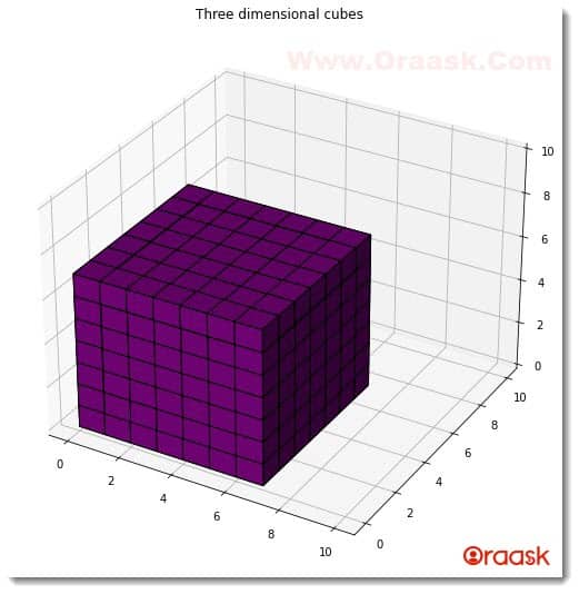
Output:

Explanation:

1. First, we imported the necessary libraries and packages in our code using the import statement of python. We imported matplotlib.pyplot and numpy libraries in our code. Next, we created a user-defined function named cubes (), which takes only one argument: side. Under this function, we first defined the dimensions of the axes using the np.indices(). We have set the dimensions of the axes to be 10,10,10. Next, we used the following lines of codes to define the dimensions of the cubes required:
2. cube = (x < side) & (y < side) & (z < side)
3. Next, we stored the value of the cube variable into the voxelarray. We set colors to the cube using the np.empty() function. This function will generate numbers corresponding to the RGB color formats. We created the figure class using the plt.figure() function and the add_subplot() function to define the axes object. We also used the projection=”3d” attribute to obtain a three-dimensional plot in the figure.
4. We also set the title to the graph using the title () function of the matplotlib.pyplot() module. We used the plt.show() function to display the graph. However, in Jupyter Notebook, this is optional to use.
5. Next, we created this main () function. This is the main part of the program. Under this function, we first defined the side of the cube. We then called the cubes () function and passed the sides variable to this function as the argument.
6. Finally, we declared the main () function as the driving code of the program using the following lines of codes:

if __name__ == “__main__”:

    main ()

Conclusion

In this article, we learned how to plot cubes in three dimensions. We have learned about the associated attributes and functions in the codes. We used the numpy and matplotlib libraries to plot the graphs. We used the functions like np.empty(), np.ones() etc. to create the data points in the code. We used the volxels () function to generate the cubes in the figures.

Although we discussed most of the critical attributes and functions in the article, we strongly recommend that the readers look up the matplotlib python documentation for more information about the associated attributes and functions.