Mathematicians use quite a large number of coordinate systems for different purposes. This includes the field of science, engineering, etc. Although while plotting the data, we mainly use the rectangular coordinate system, in many fields of science and mathematics, we need to use other coordinates for the computation and visualizations. For example, cylindrical coordinates and spherical coordinates are used in the field of electrical engineering. This article will discuss how to use the matplotlib polar plot.

Prerequisite:

Before we learn the codes, it is essential to understand the basics of matplotlib polar. We expect the readers to have sound knowledge of polar coordinates.

We recommend the readers go through the following link to understand the polar coordinates if not understood properly.”

For plotting the data and for associated works, we need some libraries. Ensure you have matplotlib and numpy installed. If not installed, open PowerShell if you are a windows user or bash terminal if you are a macOS user. Then type the following commands and hit enter:

Pip install matplotlib numpy

Parameters Required For Plotting The Polar Plot

Just like the rectangular coordinate system required x, y, and z values to be defined for plotting the figure. In the polar plot, we need to define the radius or the data point’s distance from the center of the figure and the angle subtended by the line connecting the center with the data point.

Unlike the rectangular system, we need to define the radius, angles, etc., in this system.

Plotting Scatter Plot In Polar Coordinates

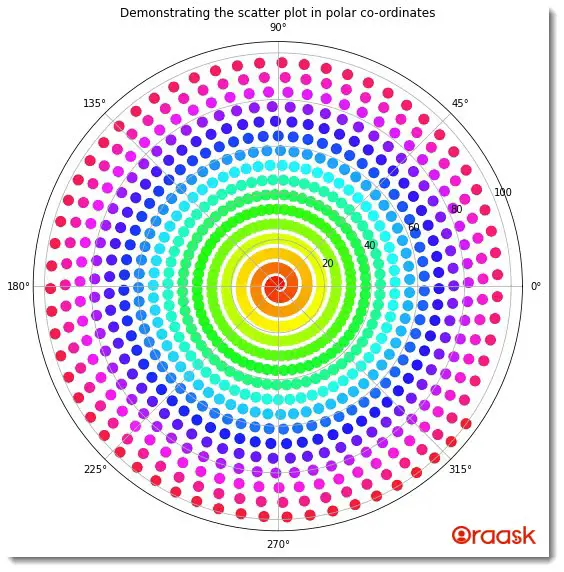
We can plot to scatter plots in polar coordinates with the help of available matplotlib functions. We first must define the coordinate system to polar using the projection attributes. Next, we need to define the angle values and the distance of the data points from the center of the plot. We can finally plot the data with the help of the scatter() function of matplotlib. We can also use other functions and attributes of the scatter() function, which we use for the rectangular coordinates.

Example (1)

# import all the necessary libraries and packages in the code
import numpy as np
import matplotlib.pyplot as plt
# creating a user-defined function named scatter
def scatter(distance, theta, colors, area):
    # creating the figure object
    fig = plt.figure(figsize=(9, 9))
    # creating the axis object and setting the projection to be polar
    ax = fig.add_subplot(projection='polar')
    # plotting the graph
    c = ax.scatter(theta, distance, c=colors, s=area, cmap='hsv', alpha=0.90)
    # Defining the title of the plot
    plt.title("Demonstrating the scatter plot in polar co-ordinates")
    # Displaying the plot
    plt.show()
# creating the main() function
def main():
    # Using arange function to set the distance
    distance = np.arange(1, 100, 0.1)
    # Creating 600 data points for the angle subtended by the points
    theta = np.arange(1, 100, 0.1)
    # Defining the area of the points to be displayed
    area = 100
    # Defining color values to be used for cmap
    colors = theta
    # Prining the data point for a better understanding
    print(theta[:100])
    print(distance[:100])
    # calling the scatter() function
    scatter(distance, theta, colors, area)
# calling the main() function
if __name__ == '__main__':
    main()

Output:

[ 1. 1.1 1.2 1.3 1.4 1.5 1.6 1.7 1.8 1.9 2. 2.1 2.2 2.3

2.4 2.5 2.6 2.7 2.8 2.9 3. 3.1 3.2 3.3 3.4 3.5 3.6 3.7

3.8 3.9 4. 4.1 4.2 4.3 4.4 4.5 4.6 4.7 4.8 4.9 5. 5.1

5.2 5.3 5.4 5.5 5.6 5.7 5.8 5.9 6. 6.1 6.2 6.3 6.4 6.5

6.6 6.7 6.8 6.9 7. 7.1 7.2 7.3 7.4 7.5 7.6 7.7 7.8 7.9

8. 8.1 8.2 8.3 8.4 8.5 8.6 8.7 8.8 8.9 9. 9.1 9.2 9.3

9.4 9.5 9.6 9.7 9.8 9.9 10. 10.1 10.2 10.3 10.4 10.5 10.6 10.7

10.8 10.9]

[ 1. 1.1 1.2 1.3 1.4 1.5 1.6 1.7 1.8 1.9 2. 2.1 2.2 2.3

2.4 2.5 2.6 2.7 2.8 2.9 3. 3.1 3.2 3.3 3.4 3.5 3.6 3.7

3.8 3.9 4. 4.1 4.2 4.3 4.4 4.5 4.6 4.7 4.8 4.9 5. 5.1

5.2 5.3 5.4 5.5 5.6 5.7 5.8 5.9 6. 6.1 6.2 6.3 6.4 6.5

6.6 6.7 6.8 6.9 7. 7.1 7.2 7.3 7.4 7.5 7.6 7.7 7.8 7.9

8. 8.1 8.2 8.3 8.4 8.5 8.6 8.7 8.8 8.9 9. 9.1 9.2 9.3

9.4 9.5 9.6 9.7 9.8 9.9 10. 10.1 10.2 10.3 10.4 10.5 10.6 10.7

10.8 10.9]

Explanation:

1. First, we imported the libraries in our code using the import statement of python. We imported the names using aliasing for convenience in our code.
2. Next, we created a user-defined function named scatter(). This void function takes four arguments: distance, theta, colors, and area. Under the function, we first created the figure object. We specified the size of the figure using the figsize attribute.
3. Next, we created the axes object using the axes() function of matplotlib. We specified the attribute projection=” polar” to specify that we will plot a polar plot. Next, we plotted the polar plot using the ax.scatter() function. Note that we used the scatter() function to plot the scatter plot. We passed the value of theta and distance to this function. We also specified the figure’s color using the c argument of the matplotlib. Then, we specified the area using the s argument and passed the area parameter as its value. We used the alpha attribute to control the intensity of the color used.
4. We specified the title of the plot using the title() function.
5. Next, we created the main() function, which is the main driving code of the program. Under this function, we first create the data point for the distance of the data points from the center of the plot. We used the arrange() function to create the data points. The function takes three parameters, called start, stop and step. The start defines the number with which iteration should start. The stop defines the number up to which iteration should take place. Next, we created an area variable and defined the area of the scattered points we used.
6. To understand the plot better, we have printed the first 100 arguments of the theta and the distance arrays. We called the scatter() function to plot the figure.
7. Finally, we called the main() function using the following lines of codes: if __name__ == ‘main‘: main()

Check This: There is a full guide on Matplotlib Polar Plot if you want to know more about Polar plot like (What it is and a lot more examples of it).

Plotting specific plot

So, we understood how to plot the figures in a polar plot. Now let us step up to plot different standard polar plots.

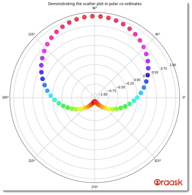
Plotting sine function in the polar plot

Example (2)

# Import all the necessary libraries and packages in the code
import numpy as np
import matplotlib.pyplot as plt
# Creating a user-defined function named scatter
def scatter(distance, theta, colors, area):
    # Creating the figure object
    fig = plt.figure(figsize=(9, 9))
    # Creating the axis object and setting the projection to be polar
    ax = fig.add_subplot(projection='polar')
    # Plotting the graph
    c = ax.scatter(distance, theta, c=colors, s=area, cmap='hsv', alpha=0.80)
    # Defining the title of the plot
    plt.title("Demonstrating the scatter plot in polar co-ordinates")
    # Displaying the plot
    plt.show()
# creating the main() function


def main():
    # Defining random seed to that the numbers are not changed each time we refresh the code
    np.random.seed(42)
    # Using arrange function to set the distance
    distance = np.arange(0, 2*np.pi, 0.1)
    # Creating 600 data points for the angle subtended by the points
    theta = np.sin(distance)
    # Defining the area of the points to be displayed
    area = 200
    # Defining color values to be used for cmap
    colors = theta
    # Printing the data point for a better understanding
    print(theta[:100])
    print(distance[:100])
    # calling the scatter() function
    scatter(distance, theta, colors, area)
# calling the main() function
if __name__ == '__main__':
    main()

Output:

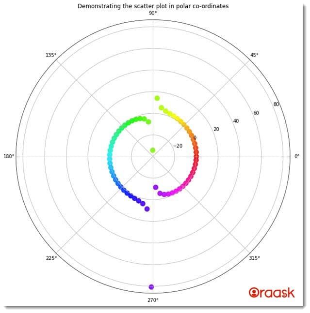
Plotting Scattered Tangent Function In A Polar Plot

Example (3)

# import all the necessary libraries and packages in the code
import numpy as np
import matplotlib.pyplot as plt
# creating a user-defined function named scatter


def scatter(distance, theta, colors, area):
    # creating the figure object
    fig = plt.figure(figsize=(9, 9))
    # creating the axis object and setting the projection to be polar
    ax = fig.add_subplot(projection='polar')
    # plotting the graph
    c = ax.scatter(distance, theta, c=colors, s=area, cmap='hsv', alpha=0.90)
    # Defining the title of the plot
    plt.title("Demonstrating the scatter plot in polar co-ordinates")
    # Displaying the plot
    plt.show()
# creating the main() function
def main():
    # defining random seed to that the numbers are not changed each time we refresh the code
    np.random.seed(42)
    # using the random function to set the distance
    distance = np.arange(0, 2*np.pi, 0.1)
    # creating 600 data points for the angle subtended by the points
    theta = np.tan(distance)
    # defining the area of the points to be displayed
    area = 100
    # defining color values to be used for cmap
    colors = distance
    # calling the scatter() function
    scatter(distance, theta, colors, area)
# calling the main() function
if __name__ == '__main__':
    main()

Output:

Check This: Article on How to Label Each Point in Scatter Plot Matplotlib if you want to know more about labeling points in a scatter plot with practical examples.

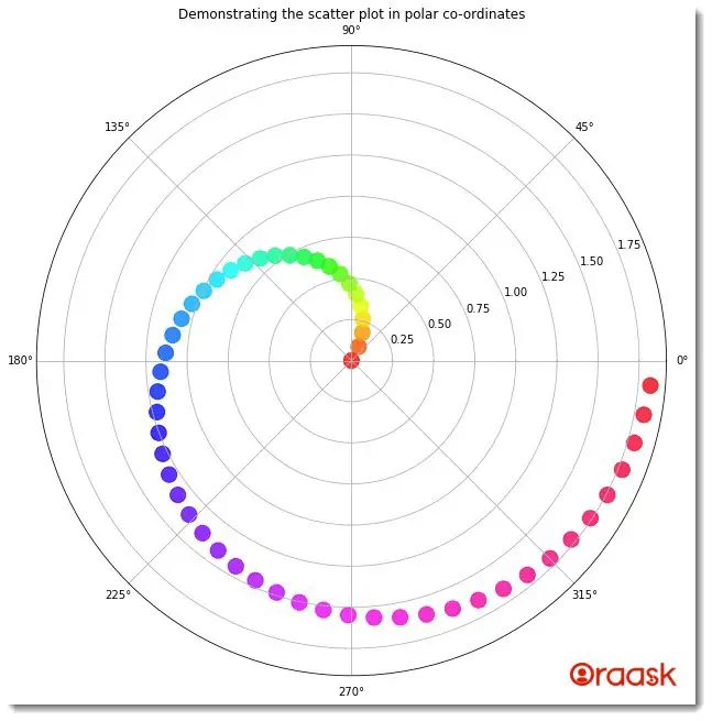
Plotting Scattered Logarithmic Graph In A Polar Plot

Example (4)

# import all the necessary libraries and packages in the code
import numpy as np
import matplotlib.pyplot as plt
# Creating a user-defined function named scatter
def scatter(distance, theta, colors, area):
    # Creating the figure object
    fig = plt.figure(figsize=(9, 9))
    # Creating the axis object and setting the projection to be polar
    ax = fig.add_subplot(projection='polar')
    # plotting the graph
    c = ax.scatter(distance, theta, c=colors, s=area, cmap='hsv', alpha=0.80)
    # Defining the title of the plot
    plt.title("Demonstrating the scatter plot in polar co-ordinates")
    # Displaying the plot
    plt.show()
# Creating the main() function
def main():
    # Defining random seed to that the numbers are not changed each time we refresh the code
    np.random.seed(42)
    # Using the random function to set the distance
    distance = np.arange(1, 2*np.pi, 0.1)
    # Creating 600 data points for the angle subtended by the points
    theta = np.log(distance)
    # Defining the area of the points to be displayed
    area = 200
    # Defining color values to be used for cmap
    colors = theta
    # Prining the data point for a better understanding
    print(theta[:100])
    print(distance[:100])
    # calling the scatter() function
    scatter(distance, theta, colors, area)
# calling the main() function
if __name__ == '__main__':
    main()

Output:

[0. 0.09531018 0.18232156 0.26236426 0.33647224 0.40546511

0.47000363 0.53062825 0.58778666 0.64185389 0.69314718 0.74193734

0.78845736 0.83290912 0.87546874 0.91629073 0.95551145 0.99325177

1.02961942 1.06471074 1.09861229 1.13140211 1.16315081 1.19392247

1.22377543 1.25276297 1.28093385 1.30833282 1.33500107 1.36097655

1.38629436 1.41098697 1.43508453 1.45861502 1.48160454 1.5040774

1.5260563 1.54756251 1.56861592 1.58923521 1.60943791 1.62924054

1.64865863 1.66770682 1.68639895 1.70474809 1.7227666 1.74046617

1.75785792 1.77495235 1.79175947 1.80828877 1.82454929]

[1. 1.1 1.2 1.3 1.4 1.5 1.6 1.7 1.8 1.9 2. 2.1 2.2 2.3 2.4 2.5 2.6 2.7

2.8 2.9 3. 3.1 3.2 3.3 3.4 3.5 3.6 3.7 3.8 3.9 4. 4.1 4.2 4.3 4.4 4.5

4.6 4.7 4.8 4.9 5. 5.1 5.2 5.3 5.4 5.5 5.6 5.7 5.8 5.9 6. 6.1 6.2]

Conclusion

This article taught us how to plot to scatter plots in polar coordinates. We specified the projection of the plot to “polar” and plotted to scatter into it using the scatter() function.

We covered all the basics of the topics required to plot a polar scatter plot. We strongly recommend that the readers use the python matplotlib documentation to understand the topic more.