The surface graph is a three-dimensional representation of python. As the name suggests, it represents a functional relationship between two independent variables, say x and z, and the value of y represents the functional value itself. This plot is very similar to the wireframe plot except for the fact that, unlike the wireframe plot, the points are filled with respective polygon figures. Such plots are extensively used in the field of mathematics and economics et where there is a requirement for plotting functions of more than one variable.

This article will explain how to plot the surface graph in three dimensions.

Creating the Surface Plot

The surface () function can do the surface plot in three dimensions in python matplotlib. Three parameters are essential for this function. They are the values of x, y, and z, respectively. Other parameters are optional, and we are free to choose from them.

Associated Functions and Attributes

• x, y, z: These attributes are mandatory. They pass the data points that must plot in the graph.
• norm: We use this attribute to normalize the values of the color map if used with it.
• vmax: We use this attribute to set the maximum value f the map required in the figure.
• vmin: This attribute sets the minimum value of the map required in the figure.
• shade: If set to true, we use this attribute to shade the face colors of the map.
• visible: This attribute defines whether the graph traces should be visible or not. The default value is “True”. This attribute takes Boolean values only.
• opacity: This attribute sets the opacity of the surface in the figure.

Example (1)

# Import all the necessary modules and functions in the code
import numpy as np
import matplotlib.pyplot as plt
# Create a user-defined function named surface()
def surface(x , y , z):
    # Next create a figure object using the figure() function
    fig = plt.figure(figsize = ( 9 , 9))
    # Creating the figure axes
    ax = plt.axes(projection = '3d')
    # Plotting the graph.
    ax.plot_surface(x, y , z, color = 'brown')
    # Defining the title of the plot
    plt.title("Surface graph")
    # Displaying the plot
    plt.show()
# Creating the main() function
def main():
    # Creating data points for the x-axis
    x = np.outer(np.linspace(-100 , 100 , 10 ) , np.ones(10))
    # Creating data points for the y axis
    y = np.linspace(-100 , 100 , 10 )
    # Creating data points for the z-axis
    z = np.sin(x ** 7) * np.cos(y ** 7)*np.tan(x**7)
    # Calling the surface() function
    surface(x, y, z)
# Calling the main() function
if __name__ == "__main__":
    main ()

Output:

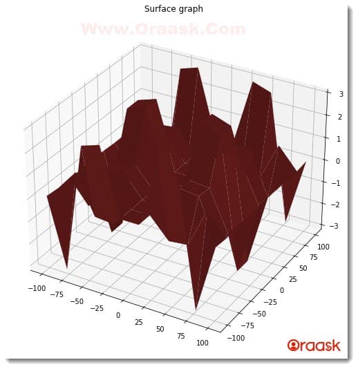
Explanation:

1. First, we imported all the necessary libraries and packages in our code using the import statement of python. We have used the alias names for convenience in our code.
2. Next, we have created a user-defined function named surface () which takes three arguments, namely x, y z. Under this function, we first created the figure object in which we specified the size of the figure using the figsize attribute. We have set the dimension of the figure to be (9,9). Next, we created the axes object. We have passed the attribute projection = “3d” in this function to specify that we want a three-dimensional space.
3. We plotted the surface graph using the plot_surface() function of python matplotlib. We have first passed the three parameters, x, y, and z, which are essential to plot the surface graph. We also specified the color of the plot as brown.
4. Next, we used the title () function to provide the title to the graph. Finally, we used the plt.show() function to display the graph. This is, however, optional in Jupyter Notebook.
5. Next, we created the main () function, which is the main driving code of the program. Under this function, we created the data points for the plot. We used the np.outer() ,np.linspace() ,np.ones() functions to create data points for the x-axis.
6. We use the np.outer()function to create multidimensional arrays. It takes two arguments. First is the number array, which should be one-dimensional. The following argument should be another array, which should be one-dimensional in shape.
7. The np.ones() function generates a numpy array with all the present elements to be one. It takes one argument that specifies the number of elements present in the array. The linspace function is used to generate data points between two numbers with some specified iterations. It takes three arguments, namely start, end and iteration. The start defines the starting number for the iteration. The end defines the last number up to which the iteration should take place, and the iteration is the iterating step of the iteration.
8. Next, we create data points for the y and z axes. Note that we used a function z= f(x , y)=sin(x ** 7) * cos(y ** 7)*tan(x**7) and implemented it in our code. Notice that the x and y are independent variables, and z here is the dependent variable on x and y. Hence it is clear that we are plotting a surface graph.
9. We called the surface function by passing the required arguments x,y, and z.
10. Finally, we called the main () function using the following lines of codes:

if __name__ == “__main__”:

        main ()

Gradient Surface Plot in Three Dimensions 3D

The gradient surface plot combines the three-dimensional surface plot and the contour plot. A contour plot is a graphical method for expressing a 3-dimensional surface that involves drawing contours on a 2-dimensional format using constant z-slice data. In such a plot, the part of the graph at a higher altitude is given different contrast of color compared to the altitude with lower heights.

Example (2)

# Import all the necessary modules and functions in the code
import numpy as np
import matplotlib.pyplot as plt
# Create a user-defined function named surface ()
def surface(x, y , z):
    colormap = plt.get_cmap('Blues')
    # Next create a figure object using the figure () function
    fig = plt.figure(figsize=( 9 , 9))
    # Creating the figure axes
    ax = plt.axes(projection = '3d')
    # Plotting the graph.
    surface_graph = ax.plot_surface(x, y, z, cmap = colormap)
    # Defining the title of the plot
    plt.title("Surface graph")
    # Defining the colorbar of the plot
    fig.colorbar(surface_graph , ax = ax , shrink=0.9 , aspect = 10)
    # Displaying the plot
    plt.show()
# Creating the main () function
def main():
    # Creating data points for the x-axis
    x = np.outer(np.linspace( -100 , 100 , 10 ), np.ones(10))
    # Creating data points for the y axis
    y = np.linspace(-100 , 100 , 10)
    # Creating data points for the z-axis
    z = np.sin(x ** 7) + np.cos( y ** 7)+np.tan(x**7)
    # Calling the surface() function
    surface(x , y , z)
# Calling the main() function
if __name__ == "__main__":
    main ()

Output:

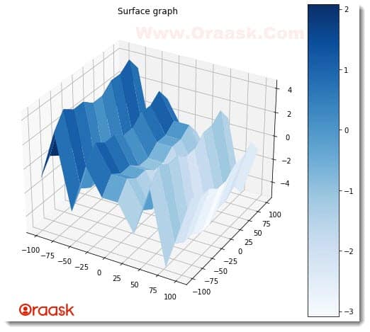
Explanation:

1. First, we imported the necessary libraries and packages in our code using the import statement of python.
2. Next, we created a user-defined function named surface () which takes three arguments: x, y, and z. Under this function, we first defined the colormap object using the get_cmap() function. We have passed the parameter “Blues” to this function. Note that this is not the same as the color argument. Look up the python matplotlib documentation to know the available values of the attributes of this function.
3. Next, we created the figure object in the code using the plt.figure() function and specified the size of the figure using the figsize() attribute.
4. Next, we created the axes object using the plt.axes() function, and we specified the attribute projection = “3d”  to specify a three-dimensional plot. Next, we plotted the graph using the ax.plot_surface() function. We first passed the necessary parameters to the code: the values of x, y, and z. We also used another attribute named the cmap and specified the value of colormap to this attribute.
5. No, we set the title to the function using the plt.title() function. We used the color bar () function to plot the color bar along the surface graph in the plot. We specified other arguments along with this function too. For example, the surface_graph is the first argument specifying which plot the colormap should belong to. The shrink specifies the size of the color bar in comparison to the height of the surface graph, and finally, the aspect specifies the aspect ratio of the color bar. The aspect ratio is defined as the length ratio to the color bar’s breadth.
6. Next, we displayed the graph using the plt.show() function.
7. After the surface () function, we created the main () function, which is the main driving code of the program. Under this function, we first created the data points. We used the numpy arrays to create data points for the x, y, and z values. We explained this in the previous code. We only changed the function in this example.
8. Next, we called the surface () function and passed the required arguments in the function.
9. We finally called the main () function using the following lines of codes:

if __name__ == “__main__”:

    main ()

Check This: There is a full guide on Matplotlib 3D Bar Chart if you want to know more about 3D Charts.

Some More Examples

Having learned how to plot the graphs, we are now ready to plot any kind of function consisting of two independent variables. We need to keep this in mind to create the data points; we should use lists or Numpy-like arrays for convenience. Also, we should take the transpose of the x matrix and store the same to the value of the y and then apply the formulae for the function to plot it in the figure. Let us now try to plot graphs depending on the specified functions.

Example (3)

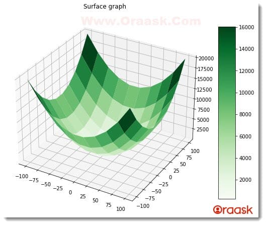
Plot the function z =  f( x , y )= x² + y²

Code:

# Import all the necessary modules and functions in the code
import numpy as np
import matplotlib.pyplot as plt
# Create a user-defined function named surface()
def surface(x, y , z):
    colormap = plt.get_cmap('Greens')
    # Next create a figure object using the figure () function
    fig = plt.figure(figsize=( 9 , 9))
    # Creating the figure axes
    ax = plt.axes(projection = '3d')
    # Plotting the graph.
    surface_graph = ax.plot_surface(x, y, z, cmap = colormap)
    # Defining the title of the plot
    plt.title("Surface graph")
    # Defining the color bar of the plot
    fig.colorbar(surface_graph , ax = ax , shrink=0.7 , aspect = 10)
    # Displaying the plot
    plt.show()
# Creating the main() function
def main():
    # Creating data points for the x-axis
    x = np.outer(np.linspace( -100 , 100 , 10 ), np.ones(10))
    # Creating data points for the y axis
    y = np.linspace(-100 , 100 , 10)
    # Creating data points for the z-axis
    z = np.power(x,2)+np.power(y,2)
    # Calling the surface() function
    surface(x , y , z)
# Calling the main() function
if __name__ == "__main__":
    main ()

Output:

Example (4)

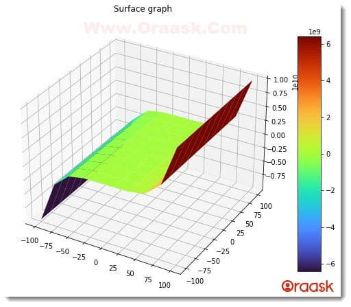
Plot the function z = f(x , y ) = x⁵ + y²

Code:

# Import all the necessary modules and functions in the code
import numpy as np
import matplotlib.pyplot as plt
# Create a user-defined function named surface()
def surface(x, y, z):
    colormap = plt.get_cmap('turbo')
    # Next create a figure object using the figure () function
    fig = plt.figure(figsize=( 9 , 9))
    # Creating the figure axes
    ax = plt.axes(projection = '3d')
    # Plotting the graph.
    surface_graph = ax.plot_surface(x, y, z, cmap = colormap)
    # Defining the title of the plot
    plt.title("Surface graph")
    # Defining the color bar of the plot
    fig.colorbar(surface_graph , ax = ax , shrink=0.7 , aspect = 10)
    # Displaying the plot
    plt.show()
# Creating the main () function
def main():
    # Creating data points for the x-axis
    x = np.outer(np.linspace( -100 , 100 , 10 ), np.ones(10))
    # Creating data points for the y axis
    y = np.linspace(-100 , 100 , 10)
    # Creating data points for the z-axis
    z = np.power(x,5)+np.power(y,2)
    # Calling the surface () function
    surface(x , y , z)
# Calling the main() function
if __name__ == "__main__":
    main()

Output:

Example (5)

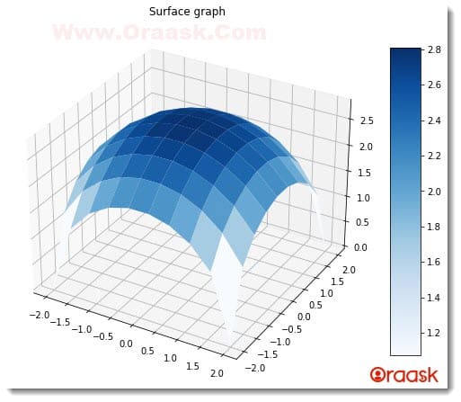
Plot the function z= f(x , y ) = 1- x² – y²

Code:

# Import all the necessary modules and functions in the code
import numpy as np
import matplotlib.pyplot as plt
# Create a user-defined function named surface()
def surface(x, y , z):
    colormap = plt.get_cmap('Blues')
    # Next create a figure object using the figure() function
    fig = plt.figure(figsize=( 9 , 9 ))
    # Creating the figure axes
    ax = plt.axes(projection = '3d')
    # Plotting the graph.
    surface_graph = ax.plot_surface(x, y, z, cmap = colormap)
    # Defining the title of the plot
    plt.title("Surface graph")
    # Defining the color bar of the plot
    fig.colorbar(surface_graph , ax = ax , shrink=0.7 , aspect = 10)
    # Displaying the plot
    plt.show()
# Creating the main () function
def main ():
    # Creating data points for the x-axis
    x = np.outer(np.linspace( -2, 2 , 10 ), np.ones(10))
    # Creating data points for the y axis
    y = x.copy().T
    # Creating data points for the z-axis
    z = np.sqrt(8-np.power(x,2)-np.power(y,2))
    # Calling the surface() function
    surface(x , y , z)

# Calling the main () function
if __name__ == "__main__":
    main ()

Output:

Conclusion:

In this article, we have learned how to plot surface graphs in a three-dimensional plot. We have discussed the surface_plot() function and the associated attributes in the code. We also learned the usage of many new functions of numpy like the np.ones() , np.linspace() , np.outer() functions in the codes .Later on, through many examples, we learned how to plot the two variable functions in matplotlib using surface graphs.

Although we have discussed most of the functions and attributes associated with the topic, we strongly recommend users go through the python matplotlib documentation to understand the associated attributes and functions more.